![]()
Structural Equation Modeling
Introduction
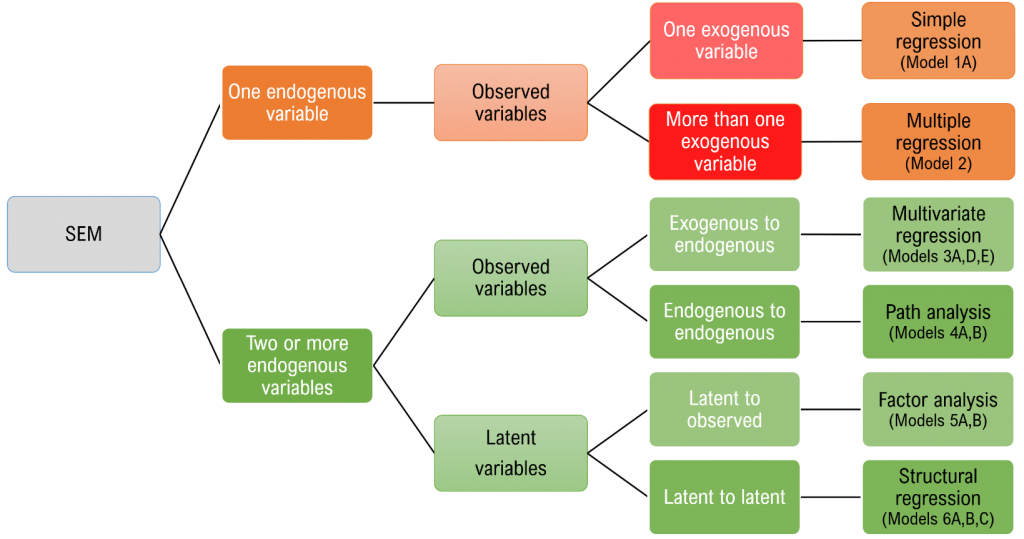
Structural Equation Modeling (SEM) is a comprehensive statistical approach that is used for testing hypotheses about the relationships among observed and latent (unobserved) variables. It combines elements of factor analysis and multiple regression analysis, allowing researchers to explore the structure of complex relationships that may exist between variables in social science, behavioral science, and other fields. Structural equation modeling is a linear model framework that models both simultaneous regression equations with latent variables. Models such as linear regression, multivariate regression, path analysis, confirmatory factor analysis, and structural regression can be thought of as special cases of SEM. The following relationships are possible in SEM:
- observed to observed variables ( \(\gamma\), e.g., regression)
- latent to observed variables ( \(\lambda\), e.g., confirmatory factor analysis)
- latent to latent variables ( \(\gamma, \beta\) e.g., structural regression)
The core components of SEM include:
Measurement Model: This part of SEM deals with the relationship between latent variables and their observed indicators. It is akin to factor analysis, where the focus is on validating the structure and loadings of observed data on latent constructs.
Structural Model: This represents the relationships between latent variables. It specifies how latent variables influence one another and can be thought of as similar to multiple regression analysis but at the level of latent constructs.
SEM is carried out in several steps:
- Model Specification: Defining the model structure, including the latent and observed variables and the hypothesized relationships between them.
- Model Identification: Ensuring that the model has enough data to estimate the relationships.
- Model Estimation: Using statistical software to estimate the parameters of the model (e.g., the strengths of the relationships between variables).
- Model Evaluation: Assessing the fit of the model to the data through various fit indices and tests (e.g., RMSEA, CFI).
- Model Modification: Based on the evaluation, the model may need adjustments to better fit the data.
- Interpretation and Reporting: Interpreting the results in the context of the research questions and reporting the findings.
SEM is powerful because it allows for the modeling of complex
relationships, including mediation and moderation effects, and can
handle measurement error more effectively than traditional regression
analysis. It requires a large sample size and is conducted using
specialized software, such as R’s lavaan package.
Broad Framework of SEM
SEM includes a range of linear models:
- Linear Regression: A basic form of statistical modeling that predicts the outcome of a dependent variable based on one or more independent variables.
- Multivariate Regression: An extension of linear regression that predicts multiple dependent variables from a set of independent variables.
- Path Analysis: Examines the directional relationships between observed variables.
- Confirmatory Factor Analysis (CFA): A specialized form of factor analysis used to test if the data fit a hypothesized measurement model.
- Structural Regression: Combines features of regression and factor analysis to model relationships between latent constructs.
The LISREL Framework: Developed by Karl Joreskög, the LISREL (linear structural relations) framework is foundational to SEM. It provides a rigorous way to parameterize these models using matrices.
Summary
- Path Analysis: It’s appropriate only for observed variables since it doesn’t include latent constructs.
- Structural Regression: It predicts relationships between latent constructs and can include observed endogenous variables as single indicator measurement models with constraints.
Path Analysis Model
Introduction
Path Analysis as a Subset of SEM: Path analysis is considered a specific instance of structural equation modeling. While both techniques are used to analyze relationships between variables, SEM encompasses a wider range of models, including those with latent variables (variables that are not directly observed but are inferred from other variables).
Assumption of Randomness: A fundamental assumption in SEM and, by extension, path analysis, is that all variables in the analysis are treated as random. This contrasts with some analytical approaches that might treat certain variables as fixed.
A simple linear regression model can be viewed as a single path model, as represented by the following simple path diagram: \[ x \longrightarrow y \leftarrow \epsilon \]
Often, the error term for an outcome (or endogenous) variable is omitted for clarity so that the following representation is equivalent: \[ x \longrightarrow y \]
Treating \(y\) and \(x\) as random variables, we can write the simple linear regression model as: \[ y=\beta_0+\beta_1 x+\epsilon \]
An implied structured covariance matrix is derived as: \[ \Sigma(\theta)=\left(\begin{array}{cc} \beta_1^2 \sigma_x^2+\sigma^2 & \beta_1 \sigma_x^2 \\ \beta_1 \sigma_x^2 & \sigma_x^2 \end{array}\right) \] where \(\theta=\left(\beta_1, \sigma^2, \sigma_x^2\right)^{\prime}\) is the parameter vector for the structured covariance matrix \(\Sigma(\theta)\).
What Does It Mean by Modeling a Covariance Structure?
In covariance structure analysis or structural equation modeling, the null hypothesis is usually of the following form: \[ H_0: \Sigma=\Sigma(\theta) \]
In common words, the equality hypothesis of the unstructured and structured population covariance matrices states that the variances and covariances of the analysis variables are exactly prescribed as functions of θ. Because the structured covariance matrix is usually derived or implied from a model, in practice this null hypothesis is equivalent to asserting that the hypothesized model is exactly true in the population.
Note: The purpose of SEM is to reproduce the variance-covariance matrix using parameters \(\theta\) we hypothesize will account for either the measurement or structural relations between variables. If the model perfectly reproduces the variance-covariance matrix then \(\Sigma=\Sigma(\theta)\).
Hypothetical-Deductive Sequence
The passage outlines a hypothetical-deductive sequence in a stepwise manner to demonstrate how SEM operates from hypothesis to data analysis: 1. Hypothesize a Model: Begin with a theoretical model that accounts for the relationships between variables. 2. Derive a Structured Covariance Matrix: From this model, derive a structured covariance matrix, \(\Sigma(\theta)\), that is hypothesized to represent the population covariance matrix. 3. Numerical Evaluation: Evaluate this structured covariance matrix using known parameter values to see if it matches the theoretical population covariance matrix.
Empirical Application
The empirical application of this sequence effectively reverses the steps, starting from observed data to test the hypothesized model: 1. Compute Sample Covariance Matrix (S): Represents the unstructured covariance matrix in the population. 2. Estimate Parameters ( \({ }^{\wedge} \theta\) ): Find the best estimates for the model parameters such that the hypothesized covariance structure, \(\Sigma\left({ }^{\wedge} \theta\right)\), matches the sample covariance matrix as closely as possible. 3. Model Assessment: Compare the hypothesized structured covariance matrix with the sample covariance matrix to assess the fit of the hypothesized model.
Path Diagram
Definitions
- observed variable: a variable that exists in the data, a.k.a item or manifest variable
- latent variable: a variable that is constructed and does not exist in the data
- exogenous variable: an independent variable either observed (x) or latent (\(\xi\)) that explains an endogenous variable
- endogenous variable: a dependent variable, either observed (y) or latent (\(\eta\)) that has a causal path leading to it
- measurement model: a model that links observed variables with latent variables
- indicator: an observed variable in a measurement model (can be exogenous or endogenous)
- factor: a latent variable defined by its indicators (can be exogenous or endogenous)
- loading: a path between an indicator and a factor
- structural model: a model that specifies causal relationships among exogenous variables to endogenous variables (can be observed or latent)
- regression path: a path between exogenous and endogenous variables (can be observed or latent)
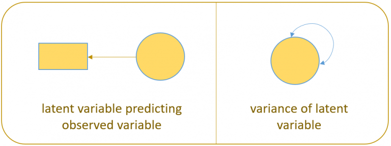
To facilitate understanding of the matrix equations (which can be a bit intimidating), a path diagram will be presented with every matrix formulation as it is a symbolic one-to-one visualization. Before we present the actual path diagram, the table below defines the symbols we will be using. Circles represent latent variables, squares represent observed indicators, triangles represent intercepts or means, one-way arrows represent paths and two-way arrows represent either variances or covariances.

For example in the figure below, the diagram on the left depicts the regression of a factor on an item (contained in a measurement model) and the diagram on the right depicts the variance of the factor (a two-way arrow pointing to a the factor itself).
The following is a path diagram of all the types of variables and relationships
Discrepancy Functions
Discrepancy functions play a critical role in parameter estimation and model fitting in structural equation modeling (SEM). They are used to measure the extent to which the sample covariance matrix \((S\) ) deviates from the model-implied covariance matrix \((\Sigma(\theta)\) ), with \(\theta\) representing the model parameters. The goal is to find the parameter values that minimize this discrepancy, indicating a good fit between the model and the observed data.
Understanding Discrepancy Functions
Discrepancy functions are essentially objective functions \((F(S, \Sigma(\theta))\) ) used in SEM to quantify the “distance” or “discrepancy” between the observed data covariance matrix and the covariance matrix predicted by the model under certain parameter values. The process involves: - Estimation: Starting with the observed covariance matrix \((S)\) and the hypothesized model structure \((\Sigma(\theta))\), the model parameters \((\theta)\) are estimated such that the discrepancy function is minimized. - Model Support: Ideally, a small minimum discrepancy function value \(\left(F_{\min }\right.\) ) supports the hypothesized model, indicating that the model-implied covariance matrix can closely reproduce the observed covariance matrix.
Common Discrepancy Functions
- Maximum Likelihood (ML) Discrepancy Function:
- \(F_{M L}(S, \Sigma(\theta))=\log |\Sigma(\theta)|-\log |S|+\operatorname{trace}\left(S \Sigma^{-1}(\theta)\right)-p\)
- Derived from the likelihood of the data under the assumption of multivariate normality.
- It includes terms for the determinants of \(S\) and \(\Sigma(\theta)\), and the trace of the product of \(S\) and the inverse of \(\Sigma(\theta)\), adjusted by the dimension \(p\).
- Normal-Theory Generalized Least Squares (NTGLS) or GLS:
- \(F_{G L S}(S, \Sigma(\theta))=\frac{1}{2} \operatorname{trace}\left[(S-\Sigma(\theta))^2\right]\)
- Assumes multivariate normality and focuses on minimizing the squared difference between \(S\) and \(\Sigma(\theta)\).
- Asymptotically Distribution-Free (ADF) or Weighted Least Squares (WLS):
- \(F_{A D F}(S, \Sigma(\theta))=\operatorname{vecs}(S-\Sigma(\theta))^{\prime} W \operatorname{vecs}(S-\Sigma(\theta))\)
- Suitable for any distribution, it minimizes the weighted squared difference, using a vector of the differences between \(S\) and \(\Sigma(\theta)\), and a weight matrix \(W\).
Choosing a Discrepancy Function
- Model Assumptions: The choice often depends on the distributional assumptions about the data. ML and GLS assume multivariate normality, while ADF/WLS does not.
- Sample Size: ADF/WLS is theoretically applicable to any distribution but requires a large sample size to achieve reliable estimates.
- Popularity and Application: Despite its assumptions, ML remains the most popular due to its balance of efficiency and robustness in practical applications.
Evaluation of the Structural Model and Goodness-of-Fit Statistics
After the estimation of model parameters, we want to make some inferential statements about the hypothesized model. There are several goodness-of-fit statistics, which are all computed after the model estimation.
In Summary, When evaluating the fit of a statistical model, especially in the context of Structural Equation Modeling (SEM), it’s crucial to use multiple goodness-of-fit indices because each index measures different aspects of model fit.
- Chi-Square \(\left(X^2\right)\) Statistic
- Purpose: Tests the null hypothesis that the model fits the data perfectly.
- Usage: A significant \(\mathrm{X}^2\) indicates a poor fit, but it is sensitive to sample size, leading to its frequent supplementation with other indices.
- Root Mean Square Error of Approximation (RMSEA)
- Purpose: Assesses the absolute fit of the model, indicating how well the model, with unknown but optimally chosen parameter estimates, would fit the population’s covariance matrix.
- Usage: Incorporates model complexity by considering degrees of freedom. Values \(\leq 0.05\) indicate a close fit, values up to 0.08 represent a reasonable error of approximation, and the \(90 \%\) confidence interval provides additional context.
- Standardized Root Mean Square Residual (SRMR)
- Purpose: Another measure of absolute fit, representing the standard deviation of the residuals between the observed and the model-implied covariance matrices.
- Usage: Values less than 0.08 are generally considered good, indicating small residuals on average.
- Comparative Fit Index (CFI)
- Purpose: Measures the incremental fit of the model compared to a baseline model, typically one of independence among variables.
- Usage: Values above 0.90 (or some suggest 0.95 for a stricter criterion) indicate a good fit to the data, considering the improvement over the null model.
- Tucker-Lewis Index (TLI)
- Purpose: Also an incremental fit index like CFI but includes a penalty for adding parameters (model complexity).
- Usage: Similar to \(\mathrm{CFI}\), values above 0.90 or 0.95 suggest a good fit.
- Akaike Information Criterion (AIC) and Bayesian Information Criterion (BIC)
- Purpose: Provide a means for model selection among a set of models, considering the goodness of fit and the number of parameters.
- Usage: They do not offer conventional cutoffs for good fit; instead, the model with the lowest AIC or BIC value among a set of models is preferred, balancing fit and complexity.
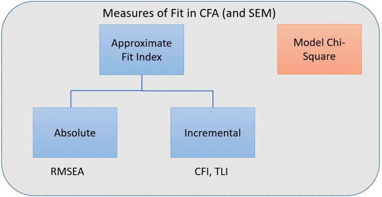
Incremental versus absolute fit index
For over-identified models, there are many types of fit indexes available to the researcher. Historically, model chi-square was the only measure of fit but in practice the null hypothesis was often rejected due to the chi-square’s heightened sensitivity under large samples. To resolve this problem, approximate fit indexes that were not based on accepting or rejecting the null hypothesis were developed. Approximate fit indexes can be further classified into a) absolute and b) incremental or relative fit indexes. An incremental fit index (a.k.a. relative fit index) assesses the ratio of the deviation of the user model from the worst fitting model (a.k.a. the baseline model) against the deviation of the saturated model from the baseline model. Conceptually, if the deviation of the user model is the same as the deviation of the saturated model (a.k.a best fitting model), then the ratio should be 1. Alternatively, the more discrepant the two deviations, the closer the ratio is to 0 (see figure below). Examples of incremental fit indexes are the CFI and TLI.
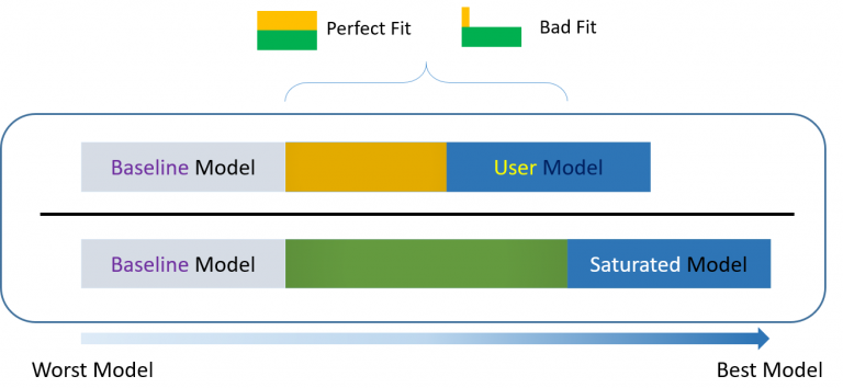
An absolute fit index on the other hand, does not compare the user model against a baseline model, but instead compares it to the observed data. An example of an absolute fit index is the RMSEA (see flowchart below).
\(\chi^2\) Test of Model Fit
The chi-square \(\left(\chi^2\right)\) statistic is computed as the product of the sample size and the minimized discrepancy function - that is \(\chi^2=N \times F_{\min }\). Some software might use \((N-1)\) in the product when only covariance structures are fitted. Recall that the null hypothesis being tested is \(H_0: \Sigma=\Sigma(\theta)\). The chi-square statistic is being used to determine whether the sample presents evidence against the null hypothesis. Under the null hypothesis of a true null model, the chi-square statistic is distributed as a \(\chi^2\) variate with specific model degrees of freedom. When the observed \(p\)-value of the chi-square statistic is very small (e.g., less than a conventional \(\alpha\)-level of 0.05), the data present an extreme event under \(H_0\). Such an extreme event (associated with a small \(p\) value) suggests that the null hypothesis \(H_0\) might not be tenable and should be rejected. Conversely, the higher the \(p\)-value associated with the observed \(\chi^2\) value, the closer the fit between the hypothesized model (under \(H_0\) ) and the perfect fit (Bollen, 1989).
However, the chi-square test statistic is sensitive to sample size. Because the \(\chi^2\) statistic equals \(N \times F_{\min }\), this value tends to be substantial when the model does not hold (even minimally) and the sample size is large (Jöreskog and Sörbom, 1993). The conundrum here, however, is that the analysis of covariance structures is grounded in large sample theory. As such, large samples are critical to obtaining precise parameter estimates, as well as to the tenability of asymptotic distributional approximations (MacCallum et al., 1996).
Findings of well-fitting hypothesized models, where the \(\chi^2\) value approximates the degrees of freedom, have proven to be unrealistic in most SEM empirical research. That is, despite relatively negligible difference between a population covariance matrix \((\Sigma)\) and a hypothesized model with population structured covariance matrix \(\Sigma(\theta)\), it is not unusual that the hypothesized model would be rejected by the \(\chi^2\) test statistic with a practically large enough sample size.
Hence, the \(\chi^2\)-testing scheme of the sharp null hypothesis \(\Sigma=\Sigma(\theta)\) in practical structural equation modeling has been deemphasized in favor of the use of various fit indices, which measures how good (or bad) the structural model approximates the truth as reflected by the unstructured model. The next few sections describe some of these popular fit indices and their conventional uses.
Loglikelihood
Two loglikelihood values are usually reported in SEM software, one for the hypothesized model (under \(H_0\) ) and the other for the saturated (or unrestricted) model (under \(H_1\) ). Some software packages might also display the loglikelihood value of the so-called baseline model-usually the uncorrelatedness model, which assumes covariances among all observed variables are zeros. Although the magnitudes of these loglikelihood values are not indicative of model fit, they are often computed because they are the basis of other fit indices such as the Information Criteria that are described in Section 1.3.4.6. Moreover, under multivariate normality, the \(\chi^2\) statistic for model fit test is -2 times of the difference between the loglikelihood values under \(H_0\) and \(H_1\).
Root Mean Square Error of Approximation (RMSEA) (Steiger and Lind, 1980) and the Standardized Root Mean Square Residual (SRMR)
They belong to the category of absolute indices of fit. However, Browne et al. (2002) have termed them, more specifically, as “absolute misfit indices” (p. 405).
By convention, RMSEA \(\leq 0.05\) indicates a good fit, and RMSEA values as high as 0.08 represents reasonable errors of approximation in the population (Browne and Cudeck, 1993). In elaborating on these cutpoints, RMSEA values ranging from 0.08 to 0.10 indicate mediocre fit, and those \(>0.10\) indicate poor fit.
The Root Mean Square Residual (RMR) represents the average residual value derived from the fitting of the variance-covariance matrix for the hypothesized model \(\Sigma(\theta)\) to the variance-covariance matrix of the sample data \((S)\). However, because these residuals are relative to the sizes of the observed variances and covariances, they are difficult to interpret. Thus, they are best interpreted in the metric of the correlation matrix ( \(\mathrm{Hu}\) and Bentler; Jöreskog and Sörbom, 1989), which is represented by its standardized version, the Standardized Root Mean Square Residual (SRMR).
The SRMR represents the average value across all standardized residuals and ranges from 0.00 to 1.00 . In a well-fitting model, this value should be small (say, . 05 or less).
Comparative Fit Index (CFI) (Bentler, 1995)
As an alternative index in model fitting, CFI is normed in the sense that it ranges from 0.00 to 1.00 , with values close to 1.00 being indicative of a wellfitting model. A cutoff value close to 0.95 has more recently been advised (Hu and Bentler, 1999). Computation of the CFI is as follows: \[ \mathrm{CFI}=1-\frac{\chi_H^2-d f_H}{\chi_B^2-d f_B} \] where \(H=\) the hypothesized model, and \(B=\) the baseline model. Usually, the baseline model refers to the uncorrelatedness model, in which the structured covariance matrix is a diagonal matrix in the population- that is, covariances among all observed variables are zeros.
Tucker-Lewis Fit Index (TLI) (Tucker and Lewis, 1973)
In contrast to the CFI, the TLI is a nonnormed index, which means that its values can extend outside the range of \(0.00-1.00\). This index is also known as Bentler’s non-normed fit index (Bentler and Bonett, 1980) in some software packages. Its values are interpreted in the same way as for the CFI, with values close to 1.00 being indicative of a well-fitting model. Computation of the TLI is as follows: \[ \mathrm{TLI}=\frac{\left(\frac{\chi_B^2}{d f_B}-\frac{\chi_H^2}{d f_H}\right)}{\left(\frac{\chi_B^2}{d f_B}-1\right)} \]
The Akaike’s Information Criterion (AIC) (Akaike, 1987) and the Bayesian Information Criterion (BIC) (Raftery, 1993; Schwarz, 1978)
The AIC and BIC are computed by the following formulas: \[ \begin{aligned} & \mathrm{AIC}=-2(\log \text {-likelihood })+2 k \\ & \mathrm{BIC}=-2(\log \text {-likelihood })+\ln (N) k \end{aligned} \] where \(\log\)-likelihood is computed under the hypothesized model \(H_0\) and \(k\) is the number of independent parameters in the model. Unlike various fit indices described previously (such as RMSEA, SRMR, CFI, and TLI), AIC and BIC are not used directly for assessing the absolute fit of a hypothesized model. Instead, AIC and BIC are mainly used for model selection.
Suppose that there are several competing models that are considered to be reasonable for explaining the data. These models can have different numbers of parameters, and they can be nested or nonnested within each other. The \(\mathrm{AIC}\) and BIC values are computed for each of these computing models. You would then select the best model, which has the smallest AIC or BIC value.
As can be seen from either formula for AIC and BIC, the first term ( -2 times of the loglikelihood) is a measure of model misfit and the second term (a multiple of the number of parameters in a model) is a measure of model complexity. Because you can always reduce, or at least never increase, model misfit (that is - minimize the first term) by increasing the model complexity with additional parameters, we can interpret AIC or BIC as a criterion that selects the best model based on the optimal balance between model fit (or misfit) and model complexity. The two information criteria differ in that the BIC assigns a greater penalty of model complexity than the AIC (say, whenever \(N \geq 8\) ), and is more apt to select parsimonious models (Arbuckle, 2007).
R lavaan Implementation
- Load Data
- Simple regression (Model 1A)
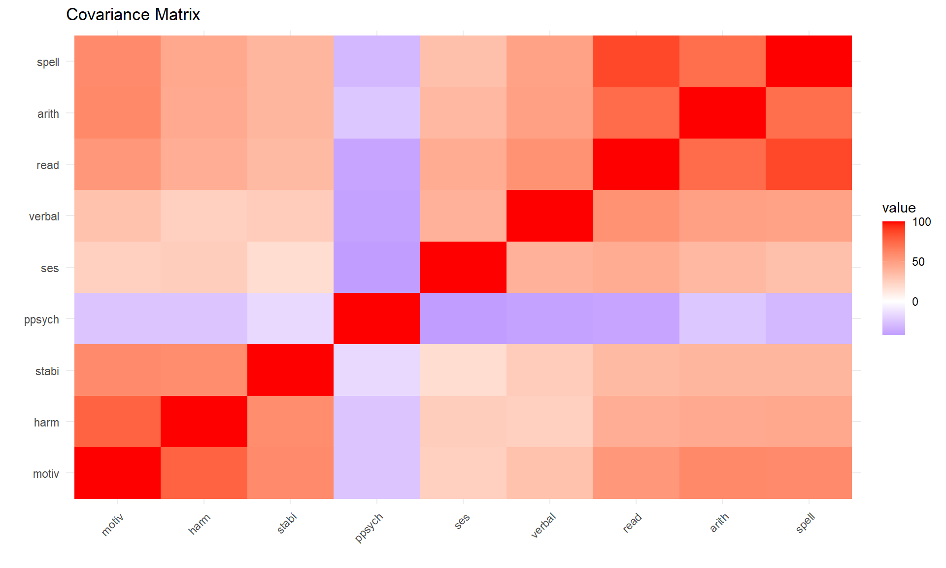
| motiv | harm | stabi | ppsych | ses | verbal | read | arith | spell | |
|---|---|---|---|---|---|---|---|---|---|
| motiv | 100 | 77 | 59 | -25.00000 | 25 | 32 | 53 | 60 | 59 |
| harm | 77 | 100 | 58 | -25.00000 | 26 | 25 | 42 | 44 | 45 |
| stabi | 59 | 58 | 100 | -16.00000 | 18 | 27 | 36 | 38 | 38 |
| ppsych | -25 | -25 | -16 | 99.99999 | -42 | -40 | -39 | -24 | -31 |
| ses | 25 | 26 | 18 | -42.00000 | 100 | 40 | 43 | 37 | 33 |
| verbal | 32 | 25 | 27 | -40.00000 | 40 | 100 | 56 | 49 | 48 |
| read | 53 | 42 | 36 | -39.00000 | 43 | 56 | 100 | 73 | 87 |
| arith | 60 | 44 | 38 | -24.00000 | 37 | 49 | 73 | 100 | 72 |
| spell | 59 | 45 | 38 | -31.00000 | 33 | 48 | 87 | 72 | 100 |
| Note: | |||||||||
| positive covariance means that as one item increases the other increases, a negative covariance means that as one item increases the other item decreases. The covariance of motiv and ppsych is -25 which means that as negative parental psychology increases student motivation decreases. |
Simple Regression
Simple regression models the relationship of an observed exogenous variable on a single observed endogenous variable. For a single subject, the simple linear regression equation is most commonly defined as:
\[ y_1=b_0+b_1 x_1+\epsilon_1 \]
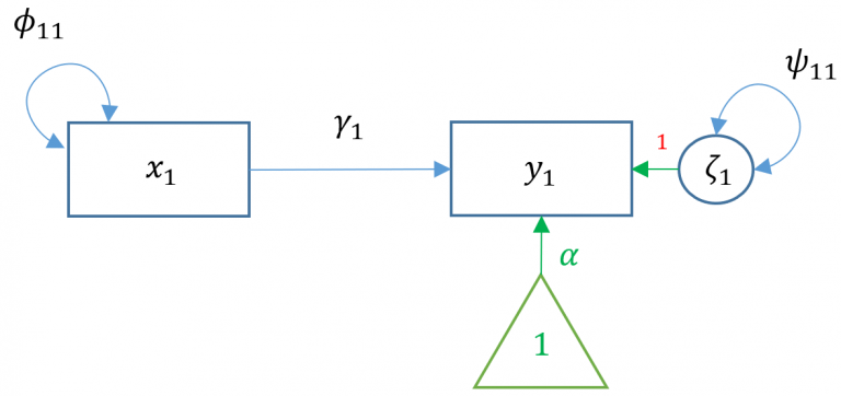
where \(b_0\) is the intercept and \(b_1\) is the coefficient and \(x\) is an observed predictor and \(\epsilon\) is the residual. Karl Joreskög, the originator of LISREL (linear structural relations), developed a special notation for the exact same model for a single observation:
\[ y_1=\alpha+\gamma x_1+\zeta_1 \]
Definitions - \(x_1\) single exogenous variable - \(y_1\) single endogenous variable - \(b_0, \alpha_1\) intercept of \(y_1\), “alpha” - \(b_1, \gamma_1\) regression coefficient, “gamma” - \(\epsilon_1, \zeta_1\) residual of \(y_1\), “epsilon” and “zeta” - \(\phi\), variance or covariance of the exogenous variable, “phi” - \(\psi\) residual variance or covariance of the endogenous variable, “psi”
To see the matrix visually, we can use a path diagram (Model 1A):
##
## Call:
## lm(formula = read ~ motiv, data = dat)
##
## Residuals:
##      Min       1Q   Median       3Q      Max
## -26.0995  -6.1109   0.2342   5.2237  24.0183
##
## Coefficients:
##               Estimate Std. Error t value Pr(>|t|)
## (Intercept) -1.232e-07  3.796e-01    0.00        1
## motiv        5.300e-01  3.800e-02   13.95   <2e-16 ***
## ---
## Signif. codes:  0 '***' 0.001 '**' 0.01 '*' 0.05 '.' 0.1 ' ' 1
##
## Residual standard error: 8.488 on 498 degrees of freedom
## Multiple R-squared:  0.2809, Adjusted R-squared:  0.2795
## F-statistic: 194.5 on 1 and 498 DF,  p-value: < 2.2e-16
## lavaan 0.6-19 ended normally after 8 iterations
##
## Estimator ML
## Optimization method NLMINB
## Number of model parameters 5
##
## Number of observations 500
##
## Model Test User Model:
##
## Test statistic 0.000
## Degrees of freedom 0
##
## Parameter Estimates:
##
## Standard errors Standard
## Information Expected
## Information saturated (h1) model Structured
##
## Regressions:
## Estimate Std.Err z-value P(>|z|)
## read ~
## motiv 0.530 0.038 13.975 0.000
##
## Intercepts:
## Estimate Std.Err z-value P(>|z|)
## .read -0.000 0.379 -0.000 1.000
## motiv 0.000 0.447 0.000 1.000
##
## Variances:
## Estimate Std.Err z-value P(>|z|)
## motiv 99.800 6.312 15.811 0.000
## .read 71.766 4.539 15.811 0.000## [1] 2.4e-07## [1] 100Intercept and Regression Coefficient
- Intercept of .read (-0.000): The notation .read signifies an endogenous variable when discussing intercepts in lavaan output. An endogenous variable is one that is influenced within the model by other variables. The intercept being -0.000 (with a small rounding error) suggests that when all predictors are at zero, the expected value of .read is essentially zero. This is consistent with linear regression models where the intercept represents the expected value of the dependent variable when all independent variables are zero.
- Regression coefficient of read ~ motiv (0.530): This coefficient represents the expected change in read (reading ability, presumably) for a one-unit increase in motiv (motivation), holding all other variables constant. The positive value suggests a positive relationship between motivation and reading ability.
Exogenous Mean and Variance
- Intercept for motiv (0.000): The absence of a dot (.) before motiv indicates it’s treated as an exogenous variable, meaning it’s assumed to influence other variables within the model but is not influenced by them. The zero intercept, after centering variables at zero, means the model assumes the average motivation level to be at this centered point.
- Variance for motiv (99.800): This closely matches the expected variance of 100, demonstrating the variability of motivation around its mean. Centering does not change variance, so this remains close to the univariate variance calculated directly from the data.
Maximum likelihood vs. least squares
The estimates of the regression coefficients are equivalent between the two methods but the variance differs. For least squares, the estimate of the residual variance is: \[ \hat{\sigma}_{L S}^2=\frac{\sum_{i=1}^N \hat{\zeta}_i^2}{N-k} \] where \(N\) is the sample size, and \(k\) is the number of predictors +1 (intercept) For maximum likelihood the estimate of the residual variance is: \[ \hat{\sigma}_{M L}^2=\frac{\sum_{i=1}^N \hat{\zeta}_i^2}{N} \]
To convert from the least squares residual variance to maximum likelihood: \[ \hat{\sigma}_{M L}^2=\left(\frac{N-k}{n}\right) \hat{\sigma}_{L S}^2 \]
- lm() output: Residual standard error: 8.488 on 498 degrees of freedom
- So the least square variance is \(8.488^2=72.046\). To convert the variance to maximum likelihood, since \(k=2\) we have \(498 / 500(72.046)=71.76\).
## [1] 71.76618Multiple Regression
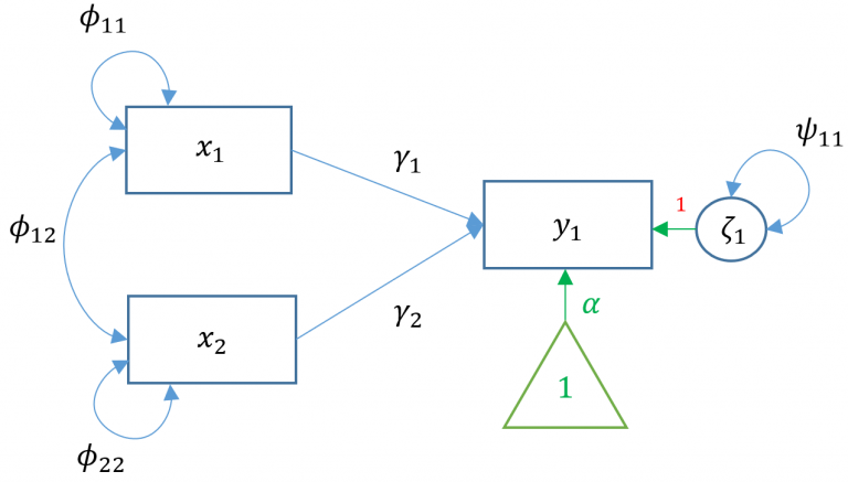
Simple regression is limited to just a single exogenous variable. In practice, a researcher may be interested in how a group of exogenous variable predict an outcome. Suppose we still have one endogenous outcome but two exogenous predictors; this is known as multiple regression (not to be confused with multivariate regression). Matrix form allows us to concisely represent the equation for all observations \[ y_1=\alpha_1+\mathbf{x} \gamma+\zeta_1 \]
Definitions - \(y_1\) single endogenous variable - \(\alpha_1\) intercept for \(y_1\) - \(\mathbf{x}\) vector \((1 \times q)\) of exogenous variables - \(\gamma\) vector \((q \times 1)\) of regression coefficients where \(q\) is the total number of exogenous variables - \(\zeta_1\) residual of \(y_1\), pronounced “zeta”. - \(\phi\), variance or covariance of the exogenous variable - \(\psi\) residual variance or covariance of the endogenous variable
Assumptions - \(E(\zeta)=0\) the mean of the residuals is zero - \(\zeta\) is uncorrelated with \(\mathbf{x}\)
Suppose we have two exogenous variables \(x_1, x_2\) predicting a single endogenous variable \(y_1\). The path diagram for this multiple regression is:
## lavaan 0.6-19 ended normally after 1 iteration
##
##   Estimator                                         ML
##   Optimization method                           NLMINB
##   Number of model parameters                         4
##
##   Number of observations                           500
##
## Model Test User Model:
##
##   Test statistic                                 0.000
##   Degrees of freedom                                 0
##
## Parameter Estimates:
##
##   Standard errors                             Standard
##   Information                                 Expected
##   Information saturated (h1) model          Structured
##
## Regressions:
##                    Estimate  Std.Err  z-value  P(>|z|)
##   read ~
##     ppsych           -0.275    0.037   -7.385    0.000
##     motiv             0.461    0.037   12.404    0.000
##
## Intercepts:
##                    Estimate  Std.Err  z-value  P(>|z|)
##    .read             -0.000    0.360   -0.000    1.000
##
## Variances:
##                    Estimate  Std.Err  z-value  P(>|z|)
##    .read             64.708    4.092   15.811    0.000
Multivariate Regression
Simple and multiple regression model one outcome \((y)\) at a time. In multivariate or simultaneous linear regression, multiple outcomes \(y_1, y_2, \ldots, y_p\) are modeled simultaneously, where \(q\) is the number of outcomes. The General Multivariate Linear Model is defined as \[ \mathbf{y}=\alpha+\mathbf{\Gamma} \mathbf{x}+\zeta \]
To see the matrix formulation more clearly, consider two (i.e., bivariate) endogenous variables \(\left(y_1, y_2\right)\) predicted by two exogenous predictors \(x_1, x_2\). \[ \left(\begin{array}{l} y_1 \\ y_2 \end{array}\right)=\left(\begin{array}{l} \alpha_1 \\ \alpha_2 \end{array}\right)+\left(\begin{array}{cc} \gamma_{11} & \gamma_{12} \\ 0 & \gamma_{22} \end{array}\right)\left(\begin{array}{l} x_1 \\ x_2 \end{array}\right)+\left(\begin{array}{l} \zeta_1 \\ \zeta_2 \end{array}\right) \]
\(\Gamma\) here is known as a structural parameter and defines the relationship of exogenous to endogenous variables.
Definitions - \(\mathbf{y}=\left(y_1, \cdots, y_p\right)^{\prime}\) vector of \(p\) endogenous variables (not the number of observations!) - \(\mathbf{x}=\left(x_1, \cdots, x_q\right)^{\prime}\) vector of \(q\) exogenous variables - \(\alpha\) vector of \(p\) intercepts - \(\Gamma\) matrix of regression coefficients \((p \times q)\) linking endogenous to exogenous variables whose \(i\) th row indicates the endogenous variable and \(j\)-th column indicates the exogenous variable - \(\zeta=\left(\zeta_1, \cdots, \zeta_p\right)^{\prime}\) vector of \(p\) residuals (for the number of endogenous variables not observations)
Multivariate regression with default covariance
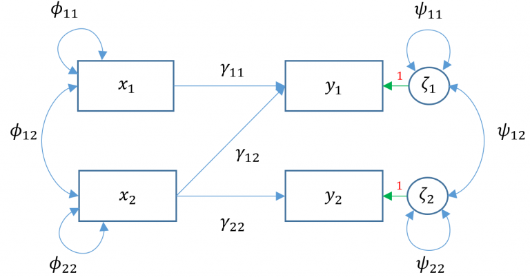
Here \(x_1\) ppsych and \(x_2\) motiv predict \(y_1\) read and only \(x_2\) motiv predicts \(y_2\) arith. The parameters \(\phi_{11}, \phi_{22}\) represent the variance of the two exogenous variables respectively and \(\phi_{12}\) is the covariance. Note that these parameters are modeled implicitly and not depicted in lavaan output. The parameters \(\zeta_1, \zeta_2\) refer to the residuals of read and arith. Finally \(\psi_{11}, \psi_{22}\) represent the residual variances of read and arith and \(\psi_{12}\) is its covariance. You can identify residual terms lavaan by noting a . before the term in the output.
Note: multivariate regression is not the same as running two separate linear regressions
By default, lavaan correlates the residual variance of the endogenous variables. To make it equivalent, constrain this covariance to zero.
## lavaan 0.6-19 ended normally after 17 iterations
##
##   Estimator                                         ML
##   Optimization method                           NLMINB
##   Number of model parameters                         6
##
##   Number of observations                           500
##
## Model Test User Model:
##
##   Test statistic                                 6.796
##   Degrees of freedom                                 1
##   P-value (Chi-square)                           0.009
##
## Parameter Estimates:
##
##   Standard errors                             Standard
##   Information                                 Expected
##   Information saturated (h1) model          Structured
##
## Regressions:
##                    Estimate  Std.Err  z-value  P(>|z|)
##   read ~
##     ppsych           -0.216    0.030   -7.289    0.000
##     motiv             0.476    0.037   12.918    0.000
##   arith ~
##     motiv             0.600    0.036   16.771    0.000
##
## Covariances:
##                    Estimate  Std.Err  z-value  P(>|z|)
##  .read ~~
##    .arith            39.179    3.373   11.615    0.000
##
## Variances:
##                    Estimate  Std.Err  z-value  P(>|z|)
##    .read             65.032    4.113   15.811    0.000
##    .arith            63.872    4.040   15.811    0.000
##
## Call:
## lm(formula = read ~ ppsych + motiv, data = dat)
##
## Residuals:
## Min 1Q Median 3Q Max
## -21.7734 -5.5633 0.1389 5.3662 25.8209
##
## Coefficients:
## Estimate Std. Error t value Pr(>|t|)
## (Intercept) -1.336e-07 3.608e-01 0.000 1
## ppsych -2.747e-01 3.730e-02 -7.363 7.51e-13 ***
## motiv 4.613e-01 3.730e-02 12.367 < 2e-16 ***
## ---
## Signif. codes: 0 '***' 0.001 '**' 0.01 '*' 0.05 '.' 0.1 ' ' 1
##
## Residual standard error: 8.068 on 497 degrees of freedom
## Multiple R-squared: 0.3516, Adjusted R-squared: 0.349
## F-statistic: 134.8 on 2 and 497 DF, p-value: < 2.2e-16##
## Call:
## lm(formula = arith ~ motiv, data = dat)
##
## Residuals:
## Min 1Q Median 3Q Max
## -23.633 -5.341 -0.214 5.106 21.271
##
## Coefficients:
## Estimate Std. Error t value Pr(>|t|)
## (Intercept) -5.400e-08 3.581e-01 0.00 1
## motiv 6.000e-01 3.585e-02 16.74 <2e-16 ***
## ---
## Signif. codes: 0 '***' 0.001 '**' 0.01 '*' 0.05 '.' 0.1 ' ' 1
##
## Residual standard error: 8.008 on 498 degrees of freedom
## Multiple R-squared: 0.36, Adjusted R-squared: 0.3587
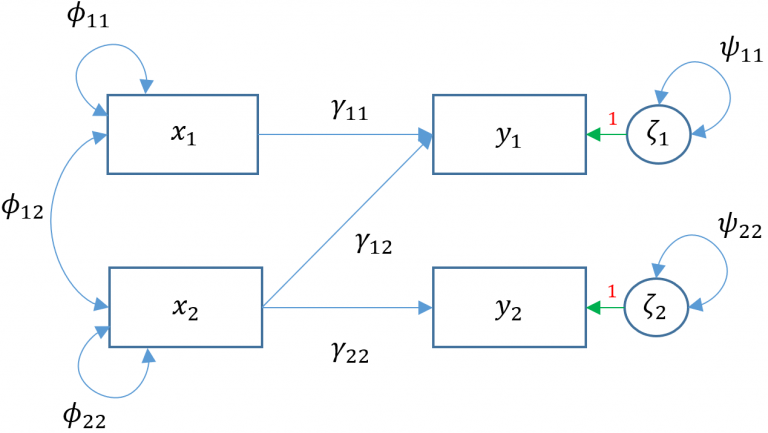
## F-statistic: 280.1 on 1 and 498 DF, p-value: < 2.2e-16Multivariate regression removing default covariances
There are two facets to the question above. We already know previously that \(1m()\) uses the least squares estimator but lavaan uses maximum likelihood, hence the difference in residual variance estimates. However, regardless of which of the two estimators used, the regression coefficients should be unbiased so there must be something else accounting for the difference in coefficients. The answer lies in the implicit fact that lavaan by default will covary residual variances of endogenous variables . read . arith. Removing the default residual covariances, we see in the path diagram
## lavaan 0.6-19 ended normally after 2 iterations
##
##   Estimator                                         ML
##   Optimization method                           NLMINB
##   Number of model parameters                         5
##
##   Number of observations                           500
##
## Model Test User Model:
##
##   Test statistic                               234.960
##   Degrees of freedom                                 2
##   P-value (Chi-square)                           0.000
##
## Parameter Estimates:
##
##   Standard errors                             Standard
##   Information                                 Expected
##   Information saturated (h1) model          Structured
##
## Regressions:
##                    Estimate  Std.Err  z-value  P(>|z|)
##   read ~
##     ppsych           -0.275    0.037   -7.385    0.000
##     motiv             0.461    0.037   12.404    0.000
##   arith ~
##     motiv             0.600    0.036   16.771    0.000
##
## Covariances:
##                    Estimate  Std.Err  z-value  P(>|z|)
##  .read ~~
##    .arith             0.000
##
## Variances:
##                    Estimate  Std.Err  z-value  P(>|z|)
##    .read             64.708    4.092   15.811    0.000
##    .arith            63.872    4.040   15.811    0.000
Fully saturated Multivariate Regression
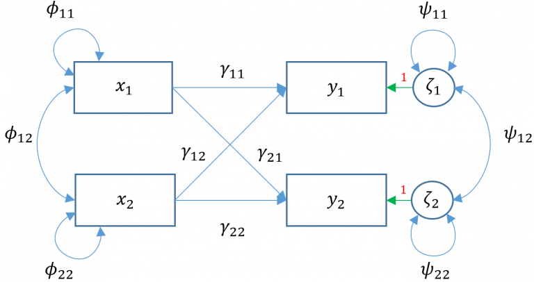
Both simple regression and multiple regression are saturated models which means that all parameters are fully estimated and there are no degrees of freedom. This is not necessarily true for multivariate regression models as Models 3A and 3B had degrees of freedom of 1 and 2 respectively.
we understand that adding a single path of \(\gamma_{21}\) turns Model 3A into a just-identified or fully saturated model which we call Model 3E.
## lavaan 0.6-19 ended normally after 39 iterations
##
##   Estimator                                         ML
##   Optimization method                           NLMINB
##   Number of model parameters                        10
##
##   Number of observations                           500
##
## Model Test User Model:
##
##   Test statistic                                 0.000
##   Degrees of freedom                                 0
##
## Parameter Estimates:
##
##   Standard errors                             Standard
##   Information                                 Expected
##   Information saturated (h1) model          Structured
##
## Regressions:
##                    Estimate  Std.Err  z-value  P(>|z|)
##   read ~
##     ppsych           -0.275    0.037   -7.385    0.000
##     motiv             0.461    0.037   12.404    0.000
##   arith ~
##     ppsych           -0.096    0.037   -2.616    0.009
##     motiv             0.576    0.037   15.695    0.000
##
## Covariances:
##                    Estimate  Std.Err  z-value  P(>|z|)
##   ppsych ~~
##     motiv           -24.950    4.601   -5.423    0.000
##  .read ~~
##    .arith            38.651    3.338   11.579    0.000
##
## Variances:
##                    Estimate  Std.Err  z-value  P(>|z|)
##     ppsych           99.800    6.312   15.811    0.000
##     motiv            99.800    6.312   15.811    0.000
##    .read             64.708    4.092   15.811    0.000
##    .arith            63.010    3.985   15.811    0.000
Path Analysis
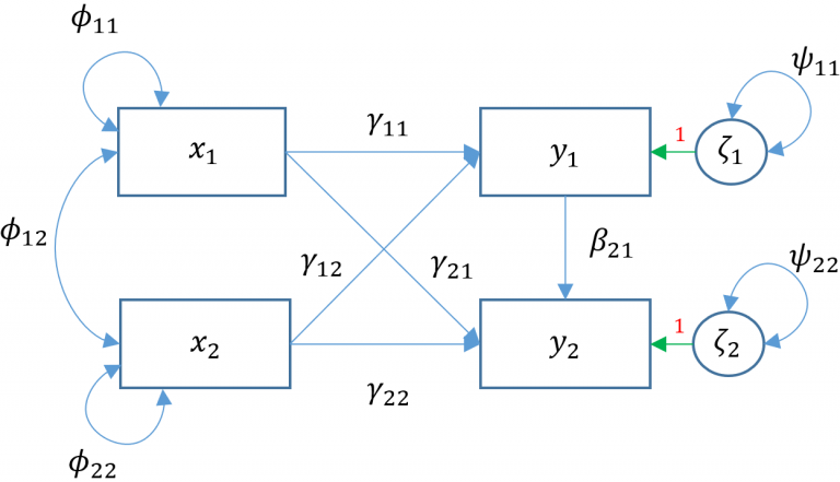
Multivariate regression is a special case of path analysis where only exogenous variables predict endogenous variables. Path analysis is a more general model where all variables are still manifest but endogenous variables are allowed to explain other endogenous variables. Since \(\Gamma\) specifies relations between an endogenous \((y)\) and exogenous \((x)\) variable, we need to create a new matrix \(B\) that specifies the relationship between two endogenous \((y)\) variables.
\[ \mathbf{y}=\alpha+\mathbf{\Gamma x}+\mathbf{B y}+\zeta \]
The matrix \(B\) is a \(p \times p\) matrix that is not necessarily symmetric. The rows of this matrix specify which \(y\) variable is being predicted and the columns specify which \(y\) ’s are predicting. For example, \(\beta_{21}\) is in the second row meaning \(y_2\) is being predicted and first column meaning \(y_1\) is predicting.
Extend our previous multivariate regression Model 3A so that we believe read which is an endogenous variable also predicts arith
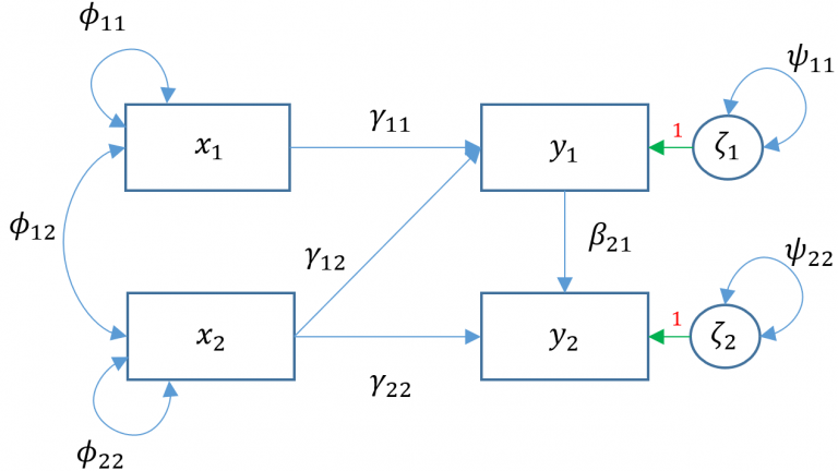
To see the matrix formulation for Model 4A, we have: \[ \left(\begin{array}{l} y_1 \\ y_2 \end{array}\right)=\left(\begin{array}{l} \alpha_1 \\ \alpha_2 \end{array}\right)+\left(\begin{array}{cc} \gamma_{11} & \gamma_{12} \\ 0 & \gamma_{22} \end{array}\right)\left(\begin{array}{l} x_1 \\ x_2 \end{array}\right)+\left(\begin{array}{cc} 0 & 0 \\ \beta_{21} & 0 \end{array}\right)\left(\begin{array}{l} y_1 \\ y_2 \end{array}\right)+\left(\begin{array}{l} \zeta_1 \\ \zeta_2 \end{array}\right) \]
Definitions - \(\mathbf{y}=\left(y_1, \cdots, y_p\right)^{\prime}\) vector of \(p\) endogenous variables - \(\mathbf{x}=\left(x_1, \cdots, x_q\right)^{\prime}\) vector of \(q\) exogenous variables - \(\alpha\) vector of \(p\) intercepts - \(\boldsymbol{\Gamma}\) matrix of regression coefficients \((p \times q)\) of exogenous to endogenous variables whose \(i\)-th row indicates the endogenous variable and \(j\)-th column indicates the exogenous variable - B matrix of regression coefficients \((p \times p)\) of endogenous to endogenous variables whose \(i\)-th row indicates the source variable and \(j\)-th column indicates the target variable - \(\zeta=\left(\zeta_1, \cdots, \zeta_p\right)^{\prime}\) vector of residuals
Assumptions - \(E(\zeta)=0\) the mean of the residuals is zero - \(\zeta\) is uncorrelated with \(x\) - \((I-B)\) is invertible (for example \(B \neq I\) )
## lavaan 0.6-19 ended normally after 1 iteration
##
##   Estimator                                         ML
##   Optimization method                           NLMINB
##   Number of model parameters                         6
##
##   Number of observations                           500
##
## Model Test User Model:
##
##   Test statistic                                 4.870
##   Degrees of freedom                                 1
##   P-value (Chi-square)                           0.027
##
## Parameter Estimates:
##
##   Standard errors                             Standard
##   Information                                 Expected
##   Information saturated (h1) model          Structured
##
## Regressions:
##                    Estimate  Std.Err  z-value  P(>|z|)
##   read ~
##     ppsych           -0.275    0.037   -7.385    0.000
##     motiv             0.461    0.037   12.404    0.000
##   arith ~
##     motiv             0.296    0.034    8.841    0.000
##     read              0.573    0.034   17.093    0.000
##
## Variances:
##                    Estimate  Std.Err  z-value  P(>|z|)
##    .read             64.708    4.092   15.811    0.000
##    .arith            40.314    2.550   15.811    0.000
## lavaan 0.6-19 ended normally after 1 iteration
##
## Estimator ML
## Optimization method NLMINB
## Number of model parameters 6
##
## Number of observations 500
##
## Model Test User Model:
##
## Test statistic 4.870
## Degrees of freedom 1
## P-value (Chi-square) 0.027
##
## Model Test Baseline Model:
##
## Test statistic 674.748
## Degrees of freedom 5
## P-value 0.000
##
## User Model versus Baseline Model:
##
## Comparative Fit Index (CFI) 0.994
## Tucker-Lewis Index (TLI) 0.971
##
## Loglikelihood and Information Criteria:
##
## Loglikelihood user model (H0) -3385.584
## Loglikelihood unrestricted model (H1) -3383.149
##
## Akaike (AIC) 6783.168
## Bayesian (BIC) 6808.456
## Sample-size adjusted Bayesian (SABIC) 6789.411
##
## Root Mean Square Error of Approximation:
##
## RMSEA 0.088
## 90 Percent confidence interval - lower 0.024
## 90 Percent confidence interval - upper 0.172
## P-value H_0: RMSEA <= 0.050 0.139
## P-value H_0: RMSEA >= 0.080 0.662
##
## Standardized Root Mean Square Residual:
##
## SRMR 0.018
##
## Parameter Estimates:
##
## Standard errors Standard
## Information Expected
## Information saturated (h1) model Structured
##
## Regressions:
## Estimate Std.Err z-value P(>|z|)
## read ~
## ppsych -0.275 0.037 -7.385 0.000
## motiv 0.461 0.037 12.404 0.000
## arith ~
## motiv 0.296 0.034 8.841 0.000
## read 0.573 0.034 17.093 0.000
##
## Variances:
## Estimate Std.Err z-value P(>|z|)
## .read 64.708 4.092 15.811 0.000
## .arith 40.314 2.550 15.811 0.000## [1] 0.0273275Path Analysis after Modification
Modification index
We see that the path analysis Model 4A as well as the multivariate regressions are over-identified models which means that their degrees of freedom is greater than zero.
Adding either of these parameters results in a fully saturated model. Without a strong a priori hypothesis, it may be difficult ascertain the best parameter to estimate. One solution is to use the modification index, which is a one degree of freedom chi-square test that assesses how the model chi-square will change as a result of including the parameter in the model. The higher the chi-square change, the bigger the impact of adding the additional parameter. To implement the modification index in lavaan, we must input into the modindices function a previously estimated lavaan model, which in this case is fit4a . The option sort=TRUE requests the most impactful parameters be placed first based on the change in chi-square.
Not all modifications to the model make sense. For example, the covariance of residuals is often times seen as an “easy” way to improve fit without changing the model. However, by adding residual covariances, you are modeling unexplained covariance between variables that by definition are not modeled by your hypothesized model. Although modeling these covariances artificially improves fit, they say nothing about the causal mechanisms your model hypothesizes.
## lavaan 0.6-19 ended normally after 1 iteration
##
##   Estimator                                         ML
##   Optimization method                           NLMINB
##   Number of model parameters                         7
##
##   Number of observations                           500
##
## Model Test User Model:
##
##   Test statistic                                 0.000
##   Degrees of freedom                                 0
##
## Parameter Estimates:
##
##   Standard errors                             Standard
##   Information                                 Expected
##   Information saturated (h1) model          Structured
##
## Regressions:
##                    Estimate  Std.Err  z-value  P(>|z|)
##   read ~
##     ppsych           -0.275    0.037   -7.385    0.000
##     motiv             0.461    0.037   12.404    0.000
##   arith ~
##     motiv             0.300    0.033    8.993    0.000
##     read              0.597    0.035   17.004    0.000
##     ppsych            0.068    0.031    2.212    0.027
##
## Variances:
##                    Estimate  Std.Err  z-value  P(>|z|)
##    .read             64.708    4.092   15.811    0.000
##    .arith            39.923    2.525   15.811    0.000
Baseline model
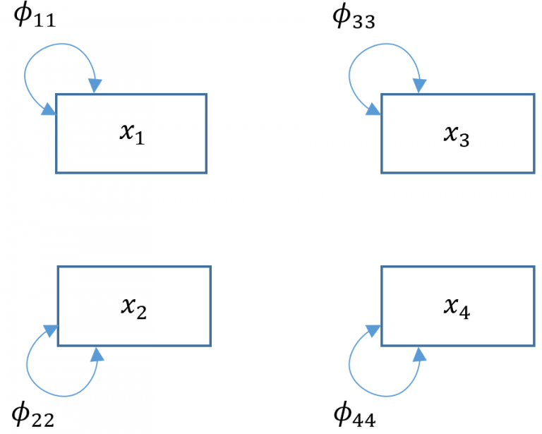
The baseline model can be thought of as the “worst-fitting” model and simply assumes that there is absolutely no covariance between variables. Suppose we modified Model 4A to become a baseline model, we would take out all paths and covariances; essentially estimating only the variances. Since there is are no regression paths, there are no endogenous variables in our model and we would only have x’s and \(\phi\)’s.
## lavaan 0.6-19 ended normally after 8 iterations
##
##   Estimator                                         ML
##   Optimization method                           NLMINB
##   Number of model parameters                         4
##
##   Number of observations                           500
##
## Model Test User Model:
##
##   Test statistic                               707.017
##   Degrees of freedom                                 6
##   P-value (Chi-square)                           0.000
##
## Model Test Baseline Model:
##
##   Test statistic                               707.017
##   Degrees of freedom                                 6
##   P-value                                        0.000
##
## User Model versus Baseline Model:
##
##   Comparative Fit Index (CFI)                    0.000
##   Tucker-Lewis Index (TLI)                       0.000
##
## Loglikelihood and Information Criteria:
##
##   Loglikelihood user model (H0)              -7441.045
##   Loglikelihood unrestricted model (H1)      -7087.537
##
##   Akaike (AIC)                               14890.091
##   Bayesian (BIC)                             14906.949
##   Sample-size adjusted Bayesian (SABIC)      14894.253
##
## Root Mean Square Error of Approximation:
##
##   RMSEA                                          0.483
##   90 Percent confidence interval - lower         0.454
##   90 Percent confidence interval - upper         0.514
##   P-value H_0: RMSEA <= 0.050                    0.000
##   P-value H_0: RMSEA >= 0.080                    1.000
##
## Standardized Root Mean Square Residual:
##
##   SRMR                                           0.380
##
## Parameter Estimates:
##
##   Standard errors                             Standard
##   Information                                 Expected
##   Information saturated (h1) model          Structured
##
## Variances:
##                    Estimate  Std.Err  z-value  P(>|z|)
##     read             99.800    6.312   15.811    0.000
##     ppsych           99.800    6.312   15.811    0.000
##     motiv            99.800    6.312   15.811    0.000
##     arith            99.800    6.312   15.811    0.000
Structural Model
Measurement Model
We have talked so far about how to model structural relationships between observed variables. A measurement model is essentially a multivariate regression model where the predictor is an exogenous or endogenous latent variable (a.k.a factor). The model is defined as
\[ \mathbf{x}=\tau_{\mathbf{x}}+\boldsymbol{\Lambda}_{\mathbf{x}} \xi+\delta \]
Definitions - \(\mathbf{x}=\left(x_1, \cdots, x_q\right)^{\prime}\) vector of \(x\)-side indicators - \(\tau_{\mathbf{x}}\) vector of \(q\) intercepts for \(x\)-side indicators - \(\xi\) vector of \(n\) latent exogenous variables - \(\delta=\left(\delta_1, \cdots, \delta_q\right)^{\prime}\) vector of residuals for \(x\)-side indicators - \(\boldsymbol{\Lambda}_{\mathbf{x}}\) matrix of loadings \((q \times n)\) corresponding to the latent exogenous variables - \(\theta_\delta\) variance or covariance of residuals for \(x\)-side indicators
The term \(\tau_{x_1}\) means the Intercept of the flrst Item, and \(\lambda_2^x\) Is the loading of the second Item wilth the factor and \(\epsilon_3\) Is the residual of the third Item, after accounting for the only factor.
Suppose we have three outcomes or \(x\)-slde Indlcators \(\left(x_1, x_2, x_3\right)\) measured by a slngle latent exogenous varlable \(\xi\). Then the path dlagram (Model 5A) for our factor model looks llke the following. Take note that the Intercepts \(\tau_{\mathbf{x}}\) are not shown but stlll modeled, and that the measurement arrows are polnting to the left.
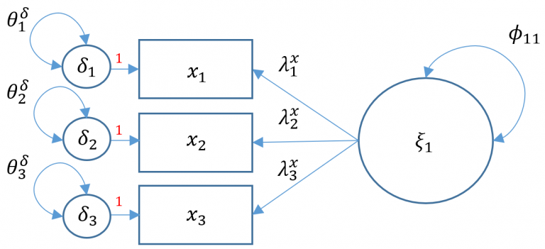
- \(\xi\) are latent exogenous variables which do not have residuals hence no residual covariances
- \(x_i\)’s are manifest exogenous variables but in fact are explained by the latent exogenous variable, therefore it has a residual term and residual variance (unexplained variance), most notably \(\theta_{\delta}\)
Exogenous Factor Analysis
Identlficatlon of the one factor model wlth three Items Is necessary due to the fact that we have 7 parameters from the modelImplled covarlance matrlx \(\Sigma(\theta)\) (e.g., three factor loadings, three resldual varlances and one factor varlance) but only \(3(4) / 2=6\) known values to work with. The extra parameter comes from the fact that we do not observe the factor but are estlmating Its varlance. In order to Identlfy a factor model with three or more Items, there are two optlons known as the marker method and the varlance standardization method. The
- marker method fixes the first loading of each factor to 1 ,
- variance standardization method fixes the variance of each factor to 1 but freely estimates all loadings.
## lavaan 0.6-19 ended normally after 37 iterations
##
##   Estimator                                         ML
##   Optimization method                           NLMINB
##   Number of model parameters                         9
##
##   Number of observations                           500
##
## Model Test User Model:
##
##   Test statistic                                 0.000
##   Degrees of freedom                                 0
##
## Parameter Estimates:
##
##   Standard errors                             Standard
##   Information                                 Expected
##   Information saturated (h1) model          Structured
##
## Latent Variables:
##                    Estimate  Std.Err  z-value  P(>|z|)   Std.lv  Std.all
##   risk =~
##     verbal            1.000                               6.166    0.617
##     ses               1.050    0.126    8.358    0.000    6.474    0.648
##     ppsych           -1.050    0.126   -8.358    0.000   -6.474   -0.648
##
## Intercepts:
##                    Estimate  Std.Err  z-value  P(>|z|)   Std.lv  Std.all
##    .verbal            0.000    0.447    0.000    1.000    0.000    0.000
##    .ses              -0.000    0.447   -0.000    1.000   -0.000   -0.000
##    .ppsych           -0.000    0.447   -0.000    1.000   -0.000   -0.000
##
## Variances:
##                    Estimate  Std.Err  z-value  P(>|z|)   Std.lv  Std.all
##    .verbal           61.781    5.810   10.634    0.000   61.781    0.619
##    .ses              57.884    5.989    9.664    0.000   57.884    0.580
##    .ppsych           57.884    5.989    9.664    0.000   57.884    0.580
##     risk             38.019    6.562    5.794    0.000    1.000    1.000
Endogenous Measurement Models
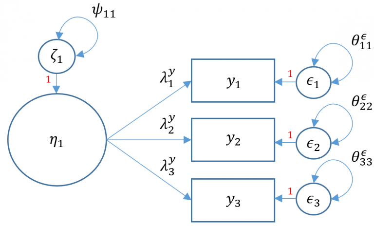
Not all latent variables are exogenous. If In the case that the latent variables Is endogenous we will rename the factor \(\eta\).
Suppose again that we have three Items except now they are labeled \(\left(y_1, y_2, y_3\right)\). For a latent endogenous variable, the structure of the measurement model remains the same except now the parameters are re-labeled as \(y\)-side variables The path diagram for Model 5B Is shown below (note, Intercepts \(\tau_{\mathbf{y}}\) are not shown but still Implicitly modeled):
In SEM, latent variables are categorized as either exogenous or endogenous:
Exogenous Latent Variables (\(x\)-side): These are the independent variables that are not influenced by other variables within the scope of the model. They can be thought of as the predictors or causes in the model. In LISREL notation, which is a software for SEM, measurement arrows for exogenous variables point to the left.
Endogenous Latent Variables (\(y\)-side): These are the dependent variables that are influenced by other variables in the model. They can be outcomes or effects. In LISREL notation, measurement arrows for endogenous variables point to the right.
\[ \mathbf{y}=\tau_{\mathbf{y}}+\mathbf{\Lambda}_{\mathbf{y}} \eta+\epsilon \]
Definitions - \(\mathbf{y}=\left(y_1, \cdots, y_p\right)^{\prime}\) vector of \(y\)-side indicators - \(\tau_{\mathbf{y}}\) vector of \(p\) intercepts for \(y\)-side indicators - \(\eta\) vector of \(m\) latent endogenous variables - \(\epsilon=\left(\epsilon_1, \cdots, \epsilon_p\right)^{\prime}\) vector of residuals for \(y\)-side indicators - \(\boldsymbol{\Lambda}_{\mathbf{y}}\) matrix of loadings \((m \times q)\) corresponding to the latent endogenous variables - \(\theta_\epsilon\) variance or covariance of residuals for \(y\)-side indicators
Differences Between Models 5A and 5B
Model 5A (Exogenous Latent Factor Analysis): This model analyzes latent factors that are not influenced by other variables within the model—essentially, it’s a factor analysis model with latent variables acting as exogenous factors.
Model 5B (Endogenous Latent Factor Analysis): This model extends Model 5A by including latent variables that act as endogenous factors, meaning they are predicted by other latent variables. This is more complex as it includes direct and indirect effects within the SEM framework.
Arrows pointing to the left indicate the measurement model for exogenous latent variables.
Arrows pointing to the right indicate the measurement model for endogenous latent variables.
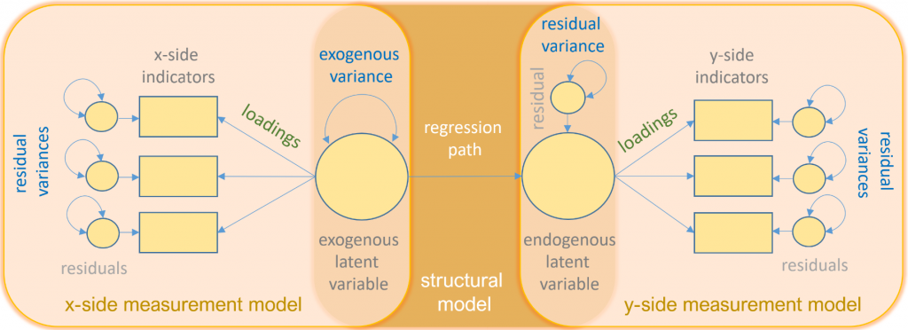
Structural Regression Model
So far we have discussed all the individual components that make up the structural regression model. Recall that multivariate regression involves regression with simultaneous endogenous variables and path analysis allows for explanatory endogenous variables. Confirmatory factor analysis is a measurement model that links latent variables to indicators. Finally, structural regression unifies the measurement and structural models to allow for explanatory latent variables, whether endogenous or exogenous.
\[ \begin{gathered} \mathbf{x}=\tau_{\mathbf{x}}+\boldsymbol{\Lambda}_{\mathbf{x}} \xi+\delta \\ \mathbf{y}=\tau_{\mathbf{y}}+\boldsymbol{\Lambda}_{\mathbf{y}} \eta+\epsilon \\ \eta=\alpha+\mathbf{B} \eta+\mathbf{\Gamma} \xi+\zeta \end{gathered} \]
Definitions Measurement variables - \(\mathbf{x}=\left(x_1, \cdots, x_q\right)^{\prime}\) vector of \(x\)-side indicators - \(\mathbf{y}=\left(y_1, \cdots, y_p\right)^{\prime}\) vector of \(y\)-side indicators - \(\tau_{\mathbf{x}}\) vector of \(q\) intercept terms for \(x\)-side indicators - \(\tau_{\mathbf{y}}\) vector of \(p\) intercept terms for \(y\)-side indicators - \(\xi\) vector of \(n\) latent exogenous variables - \(\eta\) vector of \(m\) latent endogenous variables - \(\delta=\left(\delta_1, \cdots, \delta_q\right)^{\prime}\) vector of residuals for \(x\)-side indicators - \(\epsilon=\left(\epsilon_1, \cdots, \epsilon_p\right)^{\prime}\) vector of residuals for \(y\)-side indicators - \(\boldsymbol{\Lambda}_{\mathbf{x}}\) matrix of loadings \((q \times n)\) corresponding to the latent exogenous variables - \(\mathbf{\Lambda}_{\mathbf{y}}\) matrix of loadings \((p \times m)\) corresponding to the latent endogenous variables - \(\theta_\delta\) variance or covariance of residuals for \(x\)-side indicators - \(\theta_\epsilon\) variance or covariance of residuals for \(y\)-side indicators
Structural variables - \(\alpha\) a vector of \(m\) intercepts - \(\Gamma\) a matrix of regression coefficients \((m \times n)\) of latent exogenous to latent endogenous variables whose \(i\)-th row indicates the latent endogenous variable and \(j\)-th column indicates the latent exogenous variable - \(B\) a matrix of regression coefficients \((m \times m)\) of latent endogenous to latent endogenous variables whose \(i\)-th row indicates the target endogenous variable and \(j\)-th column indicates the source endogenous variable. - \(\zeta=\left(\zeta_1, \cdots, \zeta_m\right)^{\prime}\) vector of residuals for the latent endogenous variable
Assumptlons - \(\eta\) and \(\xi\) are not observed - \(\epsilon\) and \(\delta\) are errors of measurement for \(y\) and \(x\) respectively - \(\epsilon\) is uncorrelated with \(\delta\)
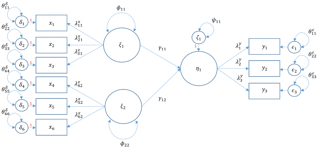
Structural regression with one endogenous variable
Just as the structural model In multivarlate regression and path analysls speclfles relatlonshlps among observed varlables, structural regresslon speclfles the relatlonshlp between latent varlables. In Model 6A, we have two latent exogenous varlables ( \(\xi_1, \xi_2\) ) predlctlng one latent endogenous varlable \(\left(\eta_1\right)\).
\[ \eta_1=\alpha_1+\left(\begin{array}{cc} \gamma_{11} & \gamma_{12} \end{array}\right)\left(\begin{array}{l} \xi_1 \\ \xi_2 \end{array}\right)+0 \cdot \eta_1+\zeta_1 \]
## lavaan 0.6-19 ended normally after 130 iterations
##
##   Estimator                                         ML
##   Optimization method                           NLMINB
##   Number of model parameters                        21
##
##   Number of observations                           500
##
## Model Test User Model:
##
##   Test statistic                               148.982
##   Degrees of freedom                                24
##   P-value (Chi-square)                           0.000
##
## Model Test Baseline Model:
##
##   Test statistic                              2597.972
##   Degrees of freedom                                36
##   P-value                                        0.000
##
## User Model versus Baseline Model:
##
##   Comparative Fit Index (CFI)                    0.951
##   Tucker-Lewis Index (TLI)                       0.927
##
## Loglikelihood and Information Criteria:
##
##   Loglikelihood user model (H0)             -15517.857
##   Loglikelihood unrestricted model (H1)     -15443.366
##
##   Akaike (AIC)                               31077.713
##   Bayesian (BIC)                             31166.220
##   Sample-size adjusted Bayesian (SABIC)      31099.565
##
## Root Mean Square Error of Approximation:
##
##   RMSEA                                          0.102
##   90 Percent confidence interval - lower         0.087
##   90 Percent confidence interval - upper         0.118
##   P-value H_0: RMSEA <= 0.050                    0.000
##   P-value H_0: RMSEA >= 0.080                    0.990
##
## Standardized Root Mean Square Residual:
##
##   SRMR                                           0.041
##
## Parameter Estimates:
##
##   Standard errors                             Standard
##   Information                                 Expected
##   Information saturated (h1) model          Structured
##
## Latent Variables:
##                    Estimate  Std.Err  z-value  P(>|z|)   Std.lv  Std.all
##   adjust =~
##     motiv             1.000                               9.324    0.933
##     harm              0.884    0.041   21.774    0.000    8.246    0.825
##     stabi             0.695    0.043   15.987    0.000    6.478    0.648
##   risk =~
##     verbal            1.000                               7.319    0.733
##     ppsych           -0.770    0.075  -10.223    0.000   -5.636   -0.564
##     ses               0.807    0.076   10.607    0.000    5.906    0.591
##   achieve =~
##     read              1.000                               9.404    0.941
##     arith             0.837    0.034   24.437    0.000    7.873    0.788
##     spell             0.976    0.028   34.338    0.000    9.178    0.919
##
## Regressions:
##                    Estimate  Std.Err  z-value  P(>|z|)   Std.lv  Std.all
##   achieve ~
##     adjust            0.375    0.046    8.085    0.000    0.372    0.372
##     risk              0.724    0.078    9.253    0.000    0.564    0.564
##
## Covariances:
##                    Estimate  Std.Err  z-value  P(>|z|)   Std.lv  Std.all
##   adjust ~~
##     risk             32.098    4.320    7.431    0.000    0.470    0.470
##
## Variances:
##                    Estimate  Std.Err  z-value  P(>|z|)   Std.lv  Std.all
##    .motiv            12.870    2.852    4.512    0.000   12.870    0.129
##    .harm             31.805    2.973   10.698    0.000   31.805    0.319
##    .stabi            57.836    3.990   14.494    0.000   57.836    0.580
##    .verbal           46.239    4.788    9.658    0.000   46.239    0.463
##    .ppsych           68.033    5.068   13.425    0.000   68.033    0.682
##    .ses              64.916    4.975   13.048    0.000   64.916    0.650
##    .read             11.372    1.608    7.074    0.000   11.372    0.114
##    .arith            37.818    2.680   14.109    0.000   37.818    0.379
##    .spell            15.560    1.699    9.160    0.000   15.560    0.156
##     adjust           86.930    6.830   12.727    0.000    1.000    1.000
##     risk             53.561    6.757    7.927    0.000    1.000    1.000
##    .achieve          30.685    3.449    8.896    0.000    0.347    0.347
Structural regression with two endogenous variables
Suppose we want to conslder a single exogenous latent varlable \(\xi_1\) predlcting two endogenous latent varlables \(\eta_1, \eta_2\) and additlonally that one of the endogenous varlables predicts another. What addltional matrlx do you think we need? SInce we have already establlshed the measurement model In \(6 \mathrm{~A}\) we can re-use the speciflcation, making note that the measurement model now has one \(x\)-slde model and two \(y\)-slde models. However, not only do we need \(\Gamma\) to model the relatlonshlp of the exogenous varlable to the two endogenous varlables, we need the \(B\) matrlx to specify the relatlonshlp of the flrst endogenous varlable to the other.
\[ \left(\begin{array}{l} \eta_1 \\ \eta_2 \end{array}\right)=\left(\begin{array}{l} \alpha_1 \\ \alpha_2 \end{array}\right)+\left(\begin{array}{l} \gamma_{11} \\ \gamma_{21} \end{array}\right) \xi_1+\left(\begin{array}{cc} 0 & 0 \\ \beta_{21} & 0 \end{array}\right)\left(\begin{array}{l} \eta_1 \\ \eta_2 \end{array}\right)+\left(\begin{array}{l} \zeta_1 \\ \zeta_2 \end{array}\right) \]
WrItIng out the equatlons we get: \[ \begin{gathered} \eta_1=\alpha_1+\gamma_{11} \xi_1+\zeta_1 \\ \eta_2=\alpha_2+\gamma_{21} \xi_1+\beta_{21} \eta_1+\zeta_2 \end{gathered} \]
The flrst equatlon speclfles that the flrst endogenous varlable is belng predlcted only by the exogenous varlable whereas the second equatlon speclfles that the second endogenous varlable is belng predicted by both the exogenous varlable and flrst endogenous varlable.
## lavaan 0.6-19 ended normally after 112 iterations
##
##   Estimator                                         ML
##   Optimization method                           NLMINB
##   Number of model parameters                        21
##
##   Number of observations                           500
##
## Model Test User Model:
##
##   Test statistic                               148.982
##   Degrees of freedom                                24
##   P-value (Chi-square)                           0.000
##
## Model Test Baseline Model:
##
##   Test statistic                              2597.972
##   Degrees of freedom                                36
##   P-value                                        0.000
##
## User Model versus Baseline Model:
##
##   Comparative Fit Index (CFI)                    0.951
##   Tucker-Lewis Index (TLI)                       0.927
##
## Loglikelihood and Information Criteria:
##
##   Loglikelihood user model (H0)             -15517.857
##   Loglikelihood unrestricted model (H1)     -15443.366
##
##   Akaike (AIC)                               31077.713
##   Bayesian (BIC)                             31166.220
##   Sample-size adjusted Bayesian (SABIC)      31099.565
##
## Root Mean Square Error of Approximation:
##
##   RMSEA                                          0.102
##   90 Percent confidence interval - lower         0.087
##   90 Percent confidence interval - upper         0.118
##   P-value H_0: RMSEA <= 0.050                    0.000
##   P-value H_0: RMSEA >= 0.080                    0.990
##
## Standardized Root Mean Square Residual:
##
##   SRMR                                           0.041
##
## Parameter Estimates:
##
##   Standard errors                             Standard
##   Information                                 Expected
##   Information saturated (h1) model          Structured
##
## Latent Variables:
##                    Estimate  Std.Err  z-value  P(>|z|)   Std.lv  Std.all
##   adjust =~
##     motiv             1.000                               9.324    0.933
##     harm              0.884    0.041   21.774    0.000    8.246    0.825
##     stabi             0.695    0.043   15.987    0.000    6.478    0.648
##   risk =~
##     verbal            1.000                               7.319    0.733
##     ses               0.807    0.076   10.607    0.000    5.906    0.591
##     ppsych           -0.770    0.075  -10.223    0.000   -5.636   -0.564
##   achieve =~
##     read              1.000                               9.404    0.941
##     arith             0.837    0.034   24.437    0.000    7.873    0.788
##     spell             0.976    0.028   34.338    0.000    9.178    0.919
##
## Regressions:
##                    Estimate  Std.Err  z-value  P(>|z|)   Std.lv  Std.all
##   adjust ~
##     risk              0.599    0.076    7.837    0.000    0.470    0.470
##   achieve ~
##     adjust            0.375    0.046    8.085    0.000    0.372    0.372
##     risk              0.724    0.078    9.253    0.000    0.564    0.564
##
## Variances:
##                    Estimate  Std.Err  z-value  P(>|z|)   Std.lv  Std.all
##    .motiv            12.870    2.852    4.512    0.000   12.870    0.129
##    .harm             31.805    2.973   10.698    0.000   31.805    0.319
##    .stabi            57.836    3.990   14.494    0.000   57.836    0.580
##    .verbal           46.239    4.788    9.658    0.000   46.239    0.463
##    .ses              64.916    4.975   13.048    0.000   64.916    0.650
##    .ppsych           68.033    5.068   13.425    0.000   68.033    0.682
##    .read             11.372    1.608    7.074    0.000   11.372    0.114
##    .arith            37.818    2.680   14.109    0.000   37.818    0.379
##    .spell            15.560    1.699    9.160    0.000   15.560    0.156
##    .adjust           67.694    6.066   11.160    0.000    0.779    0.779
##     risk             53.561    6.757    7.927    0.000    1.000    1.000
##    .achieve          30.685    3.449    8.896    0.000    0.347    0.347
Structural regression with an observed endogenous variable
See more under INTRODUCTION TO STRUCTURAL EQUATION MODELING (SEM) IN R WITH LAVAAN
Confirmatory Factor Analysis
Introduction
The CFA model commonly used for this data is the three correlated latent variables (or factors), each with three indicators as graphically described in Figure below. As seen from Figure below, these three latent factors are as follows:
- Visual factor measured by three items: x1, x2 and x3.
- Textual factor measured by three items: x4, x5 and x6.
- Speed factor measured by three items: x7, x8 and x9.
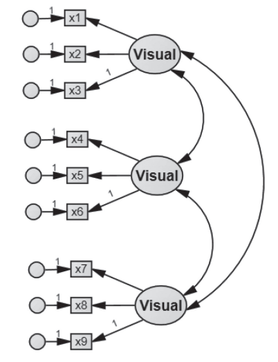
The functional relationships between the variables and the factors are prescribed by the following equations in the CFA model:
\[ \begin{aligned} & \mathrm{x} 1=b_1 \times \text { Visual }+e_1 \\ & \mathrm{x} 2=b_2 \times \text { Visual }+e_2 \\ & \mathrm{x} 3=b_3 \times \text { Visual }+e_3 \\ & \mathrm{x} 4=b_4 \times \text { Textual }+e_4 \\ & \mathrm{x} 5=b_5 \times \text { Textual }+e_5 \\ & \mathrm{x} 6=b_6 \times \text { Textual }+e_6 \\ & \mathrm{x} 7=b_7 \times \text { Speed }+e_7 \\ & \mathrm{x} 8=b_8 \times \text { Speed }+e_8 \\ & \mathrm{x} 9=b_9 \times \text { Speed }+e_9 \end{aligned} \]
In a CFA, all observed variables are endogenous, meaning that they are being explained by other variables in the system of equations. In the model equations, all observed variables appear on the left side of the equal signs. In the path diagram, all observed variables are being pointed to by latent factors and their corresponding error terms.
In a CFA, all latent factors are exogenous, meaning that they serve as explanatory variables of the outcome variables in the system of equations. In the model equations, all latent factors appear on the right side of the equal signs. In the path diagram, all latent factors are never being pointed to.
Followed from these two distinctions are two important conceptions about a CFA:
- In a CFA, the observed variables and latent factors have distinct
roles. The latent factors explain the variance and covariances of the
observed variables while the observed variables reflect or measure the
latent factors. This is why a CFA is also referred to as a measurement
model (of latent factors).
- In a CFA, the explanatory variables are latent (unobserved) in the set of linear equations so that the usual least-squares regression formulas (as described in Chapter 1) cannot be applied to estimate the factor loadings (or slope parameters). Instead, a CFA model is usually fitted by using covariance structure analysis techniques.
Two common methods to fix the scale of latent factors are:
Fixing Factor Variances to 1: This approach sets the variance of each latent factor to a constant (usually 1), which standardizes the scale of these factors.
Fixing One Loading per Factor to 1: Alternatively, one factor loading for each latent factor can be fixed to 1, establishing a reference point or scale for each factor.
Parameter Estimation
The parameters of a CFA model are consolidated into a parameter vector θ, which includes:
Factor Loadings (
bik): These parameters are arranged in the factor loading matrix \(B\). The indexing denotes that \(i\) refers to observed variables (rows of \(B\)) and \(k\) to latent factors (columns of \(B\)). These loadings indicate the extent to which each observed variable is associated with each latent factor.Factor Variances and Covariances (
ϕkl): These parameters are captured in the factor covariance matrix \(\Phi\). They represent the variance within each latent factor and the covariance between pairs of latent factors, illustrating the relationships and shared variance among them.Error Variances (\(σ^2_{ei}\)): The variances associated with measurement errors for each observed variable are the diagonal elements of the error covariance matrix \(\Psi\). These variances account for the part of observed variables’ variances not explained by the latent factors.
\
=( \[\begin{array}{ccccccccc} \sigma_{e_1}^2 & 0 & 0 & 0 & 0 & 0 & 0 & 0 & 0 \\ 0 & \sigma_{e_2}^2 & 0 & 0 & 0 & 0 & 0 & 0 & 0 \\ 0 & 0 & \sigma_{e_3}^2 & 0 & 0 & 0 & 0 & 0 & 0 \\ 0 & 0 & 0 & \sigma_{e_4}^2 & 0 & 0 & 0 & 0 & 0 \\ 0 & 0 & 0 & 0 & \sigma_{e_5}^2 & 0 & 0 & 0 & 0 \\ 0 & 0 & 0 & 0 & 0 & \sigma_{e_6}^2 & 0 & 0 & 0 \\ 0 & 0 & 0 & 0 & 0 & 0 & \sigma_{e_7}^2 & 0 & 0 \\ 0 & 0 & 0 & 0 & 0 & 0 & 0 & \sigma_{e_8}^2 & 0 \\ 0 & 0 & 0 & 0 & 0 & 0 & 0 & 0 & \sigma_{e_9}^2 \end{array}\]) $$
For the CFA model, \(\Sigma(\theta)\) can be written explicitly as a matrix expression so that the null hypothesis becomes: \[ H_0: \quad \Sigma=B \Phi B^{\prime}+\Psi \]
Reference
Chen, D.-G., & Yung, Y.-F. (2023). Structural Equation Modeling Using R/SAS: A Step-by-Step Approach with Real Data Analysis (1st ed.). Chapman and Hall/CRC. https://doi.org/10.1201/9781003365860
Jöreskog, K. G., Olsson, U. H., & Wallentin, F. Y. (2016). Multivariate analysis with LISREL. Basel, Switzerland: Springer.
Kline, R. B. (2016). Principles and practice of structural equation modeling (4th ed.). Guilford publications.
Yves Rosseel (2012). lavaan: An R Package for Structural Equation Modeling. Journal of Statistical Software, 48(2), 1-36. https://doi.org/10.18637/jss.v048.i02
INTRODUCTION TO STRUCTURAL EQUATION MODELING (SEM) IN R WITH LAVAAN
Session Info
## R version 4.4.2 (2024-10-31 ucrt)
## Platform: x86_64-w64-mingw32/x64
## Running under: Windows 10 x64 (build 19045)
##
## Matrix products: default
##
##
## locale:
## [1] LC_COLLATE=English_United States.1252
## [2] LC_CTYPE=English_United States.1252
## [3] LC_MONETARY=English_United States.1252
## [4] LC_NUMERIC=C
## [5] LC_TIME=English_United States.1252
## system code page: 65001
##
## time zone: Europe/Berlin
## tzcode source: internal
##
## attached base packages:
## [1] stats     graphics  grDevices utils     datasets  methods   base
##
## other attached packages:
##  [1] reshape2_1.4.4           lavaan_0.6-19            clinUtils_0.2.0
##  [4] htmltools_0.5.8.1        Hmisc_5.1-3              inTextSummaryTable_3.3.3
##  [7] gtsummary_2.0.3          kableExtra_1.4.0         lubridate_1.9.3
## [10] forcats_1.0.0            stringr_1.5.1            dplyr_1.1.4
## [13] purrr_1.0.2              readr_2.1.5              tidyr_1.3.1
## [16] tibble_3.2.1             ggplot2_3.5.1            tidyverse_2.0.0
##
## loaded via a namespace (and not attached):
##  [1] tidyselect_1.2.1        viridisLite_0.4.2       farver_2.1.2
##  [4] fastmap_1.2.0           fontquiver_0.2.1        digest_0.6.35
##  [7] rpart_4.1.23            timechange_0.3.0        lifecycle_1.0.4
## [10] cluster_2.1.6           magrittr_2.0.3          compiler_4.4.2
## [13] rlang_1.1.4             sass_0.4.9              tools_4.4.2
## [16] utf8_1.2.4              yaml_2.3.10             data.table_1.16.2
## [19] knitr_1.48              labeling_0.4.3          askpass_1.2.1
## [22] htmlwidgets_1.6.4       mnormt_2.1.1            plyr_1.8.9
## [25] xml2_1.3.6              withr_3.0.2             foreign_0.8-87
## [28] stats4_4.4.2            nnet_7.3-19             grid_4.4.2
## [31] fansi_1.0.6             gdtools_0.4.0           colorspace_2.1-1
## [34] MASS_7.3-61             scales_1.3.0            cli_3.6.3
## [37] rmarkdown_2.28          ragg_1.3.3              generics_0.1.3
## [40] rstudioapi_0.17.1       tzdb_0.4.0              cachem_1.1.0
## [43] parallel_4.4.2          base64enc_0.1-3         vctrs_0.6.5
## [46] jsonlite_1.8.9          fontBitstreamVera_0.1.1 hms_1.1.3
## [49] ggrepel_0.9.6           Formula_1.2-5           htmlTable_2.4.3
## [52] systemfonts_1.1.0       crosstalk_1.2.1         jquerylib_0.1.4
## [55] glue_1.8.0              cowplot_1.1.3           DT_0.33
## [58] stringi_1.8.4           flextable_0.9.7         gtable_0.3.6
## [61] quadprog_1.5-8          munsell_0.5.1           pillar_1.9.0
## [64] openssl_2.2.2           R6_2.5.1                textshaping_0.4.0
## [67] pbivnorm_0.6.0          evaluate_1.0.1          highr_0.11
## [70] haven_2.5.4             backports_1.5.0         fontLiberation_0.1.0
## [73] bslib_0.8.0             Rcpp_1.0.13             zip_2.3.1
## [76] uuid_1.2-1              svglite_2.1.3           gridExtra_2.3
## [79] checkmate_2.3.2         officer_0.6.7           xfun_0.48
## [82] pkgconfig_2.0.3