Linear Regression

Correlation Analysis

The correlation measures the strength of a linear relationship.

Pearson correlation coefficient

The Pearson correlation coefficient measures the linear relationship between two variables, X and Y. It has values between +1 and -1, where 1 indicates total positive linear correlation, 0 indicates no linear correlation, and -1 indicates total negative linear correlation. A key mathematical property of the Pearson correlation coefficient is its invariance under separate changes in the location and scale of the two variables. In other words, we can transform X to \(a + bX\) and Y to \(c + dY\) without changing the correlation coefficient, where \(a\), \(b\), \(c\), and \(d\) are constants with \(b, d > 0\). Note that more general linear transformations can, however, alter the correlation.

\[{\displaystyle \rho _{X,Y}=\operatorname {corr} (X,Y)={\operatorname {cov} (X,Y) \over \sigma _{X}\sigma _{Y}}={\operatorname {E} [(X-\mu _{X})(Y-\mu _{Y})] \over \sigma _{X}\sigma _{Y}}}\]

\[{\displaystyle \rho _{X,Y}={\operatorname {E} (XY)-\operatorname {E} (X)\operatorname {E} (Y) \over {\sqrt {\operatorname {E} (X^{2})-\operatorname {E} (X)^{2}}}\cdot {\sqrt {\operatorname {E} (Y^{2})-\operatorname {E} (Y)^{2}}}}}\]

Conditions for Applying the Pearson Correlation Coefficient:

In correlation analysis, the first consideration is whether there is likely a relationship between the two variables. If the answer is affirmative, then quantitative analysis can proceed. Additionally, the following factors must be noted (the first two are the strictest requirements, while the third is more lenient; if violated, the results tend to remain robust):

1. The Pearson correlation coefficient is suitable for cases of linear correlation. For more complex relationships, such as curvilinear correlations, the size of the Pearson correlation coefficient does not accurately represent the strength of association.

2. Extreme values in the sample can significantly impact the Pearson correlation coefficient, so careful consideration and handling are needed. If necessary, outliers can be removed or transformed to avoid erroneous conclusions due to one or two extreme values.

3. The Pearson correlation coefficient requires the variables to follow a bivariate normal distribution. It’s important to note that a bivariate normal distribution is not simply a requirement for each variable (X and Y) to be normally distributed individually but rather for them to jointly follow a bivariate normal distribution.

4. Since the Pearson correlation coefficient is calculated based on the variances and covariances of the raw data, it is sensitive to outliers and measures linear relationships. Thus, a Pearson correlation coefficient of zero only indicates no linear relationship but does not rule out other types of relationships, such as curvilinear correlation.

Spearman’s Rank Correlation Coefficient

The Spearman and Kendall correlation coefficients are both based on the relative ranks and sizes of observations, forming a more general non-parametric method that is less sensitive to outliers and therefore more robust. They primarily measure the association between variables.

Spearman’s rank correlation uses the ranks of the two variables to assess linear association and does not require any assumptions about the distribution of the original variables, making it a non-parametric statistical method. Therefore, it has a broader application range than the Pearson correlation coefficient. Spearman’s rank correlation can also be calculated for ordinal data. For data that meet Pearson’s assumptions, Spearman’s coefficient can also be calculated, although it has lower statistical efficiency and may not detect relationships as effectively as Pearson’s.

When there are no ties in the data and the two variables are perfectly monotonically related, the Spearman correlation coefficient will be +1 or -1. Even if outliers are present, they typically do not significantly impact the Spearman correlation coefficient, as outliers’ ranks tend to remain at the extremes (e.g., first or last), thus minimizing their effect on Spearman’s measure of association.

\[{\displaystyle r_{s}=\rho _{\operatorname {rg} _{X},\operatorname {rg} _{Y}}={\frac {\operatorname {cov} (\operatorname {rg} _{X},\operatorname {rg} _{Y})}{\sigma _{\operatorname {rg} _{X}}\sigma _{\operatorname {rg} _{Y}}}}}\]

Kendall’s Rank Correlation Coefficient

The Kendall rank correlation coefficient is a measure of ordinal association, suitable for reflecting the correlation between categorical variables when both variables are ordered categories. It is denoted by the Greek letter \(\tau\), and ranges between -1 and 1. When \(\tau = 1\), it indicates perfect ordinal agreement between two random variables, while \(\tau = -1\) indicates perfect ordinal disagreement. A value of \(\tau = 0\) implies that the two variables are independent.

Formula: The Kendall coefficient is based on concordance. For two pairs of observations \((X_i, Y_i)\) and \((X_j, Y_j)\), if \(X_i > X_j\) and \(Y_i > Y_j\) (or vice versa), the pair is considered concordant; otherwise, it is discordant. The Kendall correlation coefficient is calculated as follows:

\[ \tau = \frac{{\text{number of concordant pairs} - \text{number of discordant pairs}}}{{n \choose 2}} \]

where \({n \choose 2} = \frac{n(n-1)}{2}\) represents the number of ways to choose two items from \(n\) items.

Intraclass Correlation Coefficient (ICC)

When measuring quantitative characteristics in units organized into groups, the intraclass correlation coefficient (ICC) describes how similar units within the same group are to each other. Unlike most correlation measures, ICC operates on group-structured data rather than paired observations. ICC is commonly used to assess the similarity of quantitative attributes among individuals with specific familial relationships or to evaluate the consistency or reliability of measurement methods or raters for the same quantitative outcome.

Fisher’s original ICC is algebraically similar to the Pearson correlation coefficient but differs in that it centers and scales data based on a pooled mean and standard deviation across groups. This pooled scaling is meaningful for ICC because all quantities being measured are the same, although they pertain to different units in various groups.

The formula for ICC is:

\[ r = \frac{1}{Ns^2} \sum_{n=1}^{N}(x_{n,1} - \bar{x})(x_{n,2} - \bar{x}), \]

where:

\[ \bar{x} = \frac{1}{2N} \sum_{n=1}^{N}(x_{n,1} + x_{n,2}), \]

and

\[ s^2 = \frac{1}{2N} \left\{ \sum_{n=1}^{N}(x_{n,1} - \bar{x})^2 + \sum_{n=1}^{N}(x_{n,2} - \bar{x})^2 \right\}. \]

In Pearson correlation, each variable is centered and scaled by its own mean and standard deviation:

\[ r_{xy} = \frac{\sum_{i=1}^{n} \left( x_i - \bar{x} \right) \left( y_i - \bar{y} \right)}{\sqrt{\sum_{i=1}^{n} \left( x_i - \bar{x} \right)^2} \sqrt{\sum_{i=1}^{n} \left( y_i - \bar{y} \right)^2}}. \]

Visualize Correlation in R

bank<- data.frame(
  y=c(1018.4,1258.9,1359.4,1545.6,1761.6,1960.8),
  x1=c(159,42,95,102,104,108),
  x2=c(223.1,269.4,297.1,330.1,337.9,400.5),
  x3=c(500,370,430,390,330,310),
  x4=c(112.3,146.4,119.9,117.8,122.3,167.0),
  w=c(5,6,8,3,6,8)
)
cor(bank[,c(2,3,4,5)],method = "pearson")

##            x1         x2         x3         x4
## x1  1.0000000 -0.1604025  0.5095785 -0.4331830
## x2 -0.1604025  1.0000000 -0.8558009  0.5987314
## x3  0.5095785 -0.8558009  1.0000000 -0.7010598
## x4 -0.4331830  0.5987314 -0.7010598  1.0000000

## Visualize the correlation matrix
library(corrplot)
bank.cor <- cor(bank)
corrplot(bank.cor, method = "ellipse")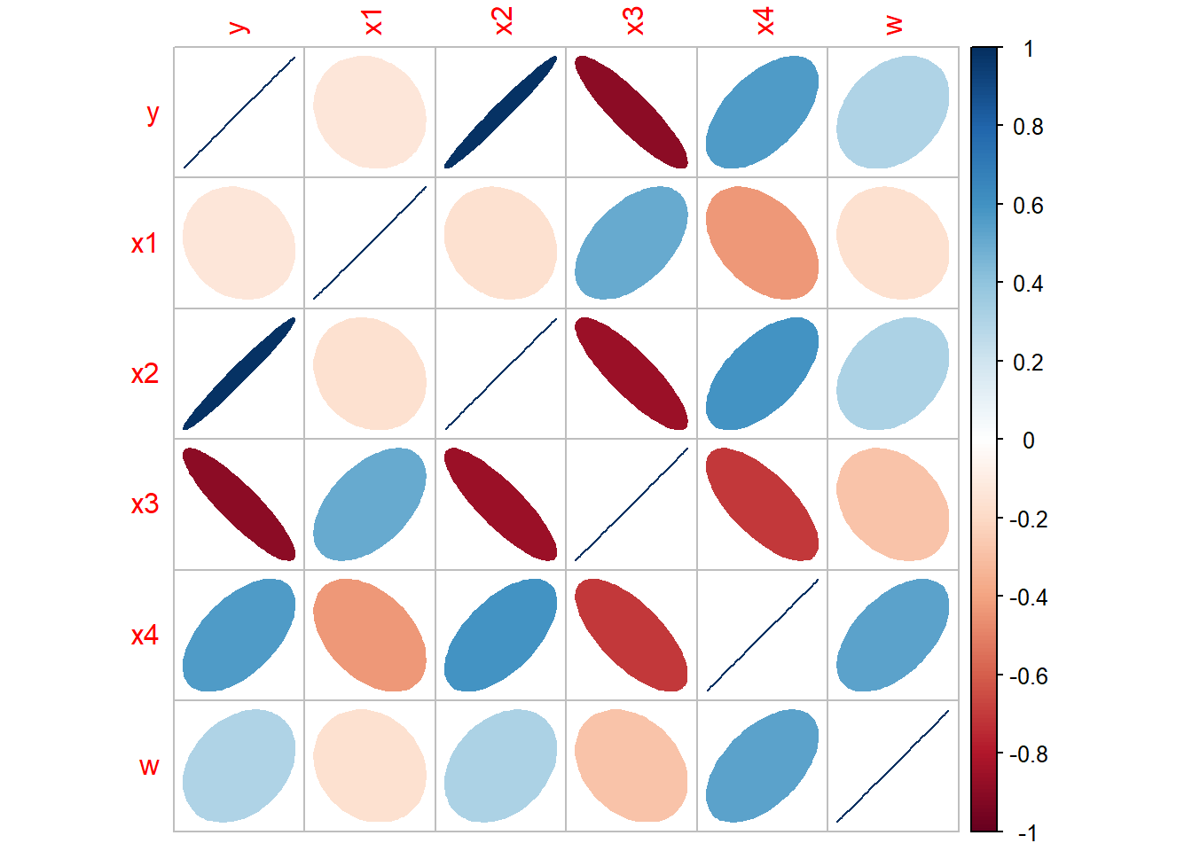

## devtools::install_github("kassambara/ggcorrplot")
library(ggplot2)
library(ggcorrplot)

## Correlation matrix
data(mtcars)
corr <- round(cor(mtcars), 1)

## Plot
ggcorrplot(corr, hc.order = TRUE, 
           type = "lower", 
           lab = TRUE, 
           lab_size = 3, 
           method="circle", 
           colors = c("tomato2", "white", "springgreen3"), 
           title="Correlogram of mtcars", 
           ggtheme=theme_bw)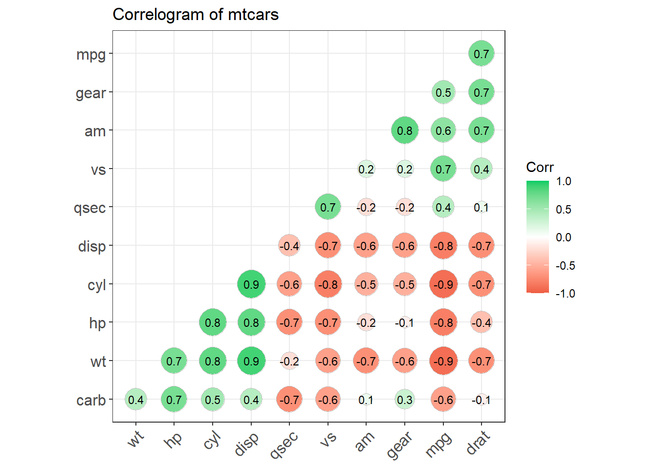

Ordinary Least Squares (OLS)

General Form of Regression Model

Linear Regression Model (Formula):

• It presents a linear regression model: \[ y = \beta_0 + \beta_1x_1 + \beta_2x_2 + \ldots + \beta_px_p + \epsilon \] where \(y\) is the dependent variable, \(x_1, x_2, \ldots, x_p\) are the independent variables, \(\beta_0, \beta_1, \ldots, \beta_p\) are coefficients to be estimated, and \(\epsilon\) is the random error term.

Objective and Estimation:

• The model’s goal is to predict the dependent variable based on the independent variables, accounting for random errors.
• The coefficients \(\beta_i\) are estimated using the OLS method, which aims to minimize the sum of squared residuals between the observed and predicted values.

Assumptions for the Gauss-Markov Theorem:

• Linearity: The relationship between the dependent and independent variables is linear.
• Independence: Observations are independent of each other.
• Homoscedasticity: Constant variance of error terms across observations.
• Zero Mean Error: The expected value of the error term is zero conditional on the independent variables.
• No Perfect Multicollinearity: There is no exact linear relationship among the independent variables.

Gauss-Markov Theorem:

• Under these assumptions, the OLS estimator is the best linear unbiased estimator, meaning it has the smallest variance among all linear unbiased estimators for the coefficients.
• if the error terms are normally distributed, this leads to additional beneficial properties for hypothesis testing regarding the regression coefficients, including t-tests and F-tests.
• The errors \(\epsilon_i\) are assumed to be normally distributed \(N(0, \sigma^2)\) and are independent and identically distributed, which simplifies the model’s analysis and inference processes.

Assumpions

\[{\displaystyle \mathbf {y} =\mathbf {X} {\boldsymbol {\beta }}+{\boldsymbol {\varepsilon }}\;} \ \ \ \ {\displaystyle \;{\boldsymbol {\varepsilon }}\sim {\mathcal {N}}(\mathbf {0} ,\sigma ^{2}\mathbf {I} _{T})}.\]

1. \(y_{i}=\alpha+\beta x_{i}+\varepsilon_{i}\)
2. \(\mathrm{E}\left(\varepsilon_{i}\right)=0\)
3. \(\operatorname{var}\left(\varepsilon_{i}\right)=\sigma^{2}\)
4. \(\operatorname{cov}\left(\varepsilon_{i}, \varepsilon_{j}\right)=0\)
5. \(\varepsilon_{i} \sim\) Normal Distribution
6. \(n>p\): number of sample size is greater than the number of explanatory variables.

Interpretation

• Linearity: The relationship between the predictor and response variables should be linear. If this relationship isn’t clearly linear, data transformations (e.g., logarithmic, polynomial, or exponential transformations) can be applied to the variables X or Y to achieve linearity.

• Uncorrelated Residuals: Residuals (errors) should be uncorrelated with each other, meaning there should be no pattern in the residuals.

• Homoscedasticity: The errors should be normally distributed and have constant variance. This implies that for different input values, the variance of the errors remains constant. If this assumption is violated, parameter estimates may become biased, leading to significance test results that are too high or too low, potentially resulting in incorrect conclusions. This situation is known as heteroscedasticity.

• Non-collinearity: There should be no linear relationship between predictor variables; predictors should ideally be independent of each other. Collinearity can lead to biased estimates.

• Outliers: Outliers can severely impact parameter estimation. Ideally, outliers should be removed before fitting a model using linear regression.

Matrix Solution

Least squares method minimum \(J\left(\theta_{0}, \theta_{1}\right)\) and find out the smallest \(\theta_{0}\) and \(\theta_{1}\)

\[J(\theta_0, \theta_1) = \sum\limits_{i=1}^{m}(y^{(i)} - h_\theta(x^{(i)})^2 = \sum\limits_{i=1}^{m}(y^{(i)} - \theta_0 - \theta_1 x^{(i)})^2\]

Assume \[h_\theta(x_1, x_2, ...x_n) = \theta_0 + \theta_{1}x_1 + ... + \theta_{n}x_{n}\] as \[h_\mathbf{\theta}(\mathbf{x}) = \mathbf{X\theta}\]

\[J(\mathbf\theta) = \frac{1}{2}(\mathbf{X\theta} - \mathbf{Y})^T(\mathbf{X\theta} - \mathbf{Y})\]

Take the derivative of the θ vector for this loss function to 0

\[\frac{\partial}{\partial\mathbf\theta}J(\mathbf\theta) = \mathbf{X}^T(\mathbf{X\theta} - \mathbf{Y}) = 0\] \[\mathbf{X^{T}X\theta} = \mathbf{X^{T}Y}\] \[\mathbf{\theta} = (\mathbf{X^{T}X})^{-1}\mathbf{X^{T}Y}\]

Gauss-Markov Theorem

The Gauss-Markov Theorem establishes that the Ordinary Least Squares (OLS) method has particularly desirable properties. Specifically, when the mean of the error terms is zero, the OLS estimator \(\hat{\beta}\) is unbiased. If the error terms also have constant variance, then OLS provides the Best Linear Unbiased Estimator (BLUE). Additionally, if the error terms in a linear regression model are uncorrelated, the OLS estimator has the lowest sampling variance among linear unbiased estimators. While \(\hat{\beta}\) is a reasonable estimator, there are other options. However, OLS is preferred for three key reasons:

1. Orthogonal Projection: OLS results from an orthogonal projection onto the model space, providing a geometrically intuitive solution.

2. Maximum Likelihood Estimator: If the errors are independent and identically normally distributed, OLS serves as the maximum likelihood estimator (MLE). In essence, the MLE for \(\hat{\beta}\) is the value that maximizes the likelihood of observing the given data.

3. Gauss-Markov Theorem: The theorem confirms that OLS provides the best linear unbiased estimate (BLUE), ensuring minimum variance within the class of linear unbiased estimators.

limitation

Limitations of Ordinary Least Squares (OLS):

1. Matrix Inversion Requirement: OLS requires calculating the inverse of \(\left(\mathbf{X}^{\mathrm{T}} \mathbf{X}\right)\). If this matrix is not invertible, OLS cannot be directly applied. In such cases, gradient descent can still be used. Alternatively, we can restructure the sample data by removing redundant features to ensure that \(\left(\mathbf{X}^{\mathrm{T}} \mathbf{X}\right)\) has a non-zero determinant, allowing OLS to proceed.

2. High Dimensionality: When the number of features (\(n\)) is very large, calculating the inverse of the \(\left(\mathbf{X}^{\mathrm{T}} \mathbf{X}\right)\) matrix (an \(n \times n\) matrix) becomes computationally expensive or even infeasible. Iterative methods, like gradient descent, remain viable in such cases. As a rule of thumb, if \(n\) exceeds 10,000 and distributed computing resources are limited, iterative methods are recommended. Alternatively, dimensionality reduction techniques, such as Principal Component Analysis (PCA), can reduce the feature space, enabling OLS to be applied.

3. Nonlinear Relationships: If the relationship between variables is not linear, OLS cannot be directly applied, as it is designed for linear models. Transforming the relationship into a linear form may allow OLS to be used, but gradient descent is a more flexible option that can handle nonlinear relationships.

4. Special Cases in Sample Size: When the number of samples (\(m\)) is very small, specifically smaller than the number of features (\(n\)), the system of equations is underdetermined, making it difficult to fit the data using standard optimization methods. When \(m = n\), the system can be solved using standard equations. If \(m > n\), the system becomes overdetermined, which is the typical scenario where OLS performs effectively.

Practical Difficulties Using OLS

When using Ordinary Least Squares (OLS) regression, several practical challenges can limit the reliability and interpretability of the results:

1. Nonrandom Samples

   The way data is collected directly affects the conclusions that can be drawn. Hypothesis testing assumes that the data is a simple random sample from a larger population. This sample should ideally be large enough to represent the population accurately but still small in proportion to the overall population size. However, if the sample is not random, statistical inference can become unreliable. For non-random samples, descriptive statistics may still be useful, but applying inferential techniques might yield misleading results, and conclusions drawn from such data are inherently less reliable.

2. Choice and Range of Predictors

   If significant predictors are omitted from the model, the model’s predictions can be poor, and it may misrepresent relationships between predictors and the response. The range and conditions of data collection can limit predictive effectiveness, and extrapolating beyond the observed range of data can be dangerous.

3. Model Misspecification

   OLS relies on assumptions about the structure of both the systematic and random components of the model. For example, it assumes that errors follow a normal distribution: \(\varepsilon \sim \mathrm{N}(0, \sigma^2 I)\). If this assumption is incorrect, or if the assumed linear structure \(E(y) = X\beta\) does not adequately represent the data, then the model’s reliability and accuracy may suffer.

4. Practical vs. Statistical Significance

   Statistical significance does not always imply practical importance. Larger sample sizes tend to produce smaller p-values, so it’s essential not to equate statistical significance with the real-world importance of predictor effects. For large datasets, statistically significant results are easier to obtain, even if the actual effect is minor or inconsequential. Confidence intervals (CIs) for parameter estimates provide a better way to assess the size of an effect. CIs remain useful even when we fail to reject the null hypothesis, as they indicate the range of plausible values and the precision of estimates, offering insight into the real effect’s potential magnitude.

Moreover, models are typically approximations of reality, making the exact interpretation of parameters open to question. As the amount of data increases, the power of tests grows, potentially detecting even trivial differences. Therefore, if we fail to reject the null hypothesis, it may simply indicate insufficient data rather than a lack of meaningful results, underscoring the importance of focusing on CIs rather than just hypothesis testing.

Here’s the modified code with a different dataset, mtcars, to demonstrate collinearity diagnostics.

# Load the mtcars dataset
data(mtcars)

# Fit a linear model
g <- lm(mpg ~ ., data = mtcars)
summary(g)

# Check the correlation matrix
round(cor(mtcars), 3)

# Check the eigendecomposition of X^T X
x <- model.matrix(g)[, -1]  # Remove intercept
e <- eigen(t(x) %*% x)
e$values  # Eigenvalues

# Condition numbers (ratio of largest eigenvalue to each eigenvalue)
sqrt(e$values[1] / e$values)

# Check the variance inflation factors (VIFs)
# For the first predictor
r_squared <- summary(lm(x[, 1] ~ x[, -1]))$r.squared
1 / (1 - r_squared)  # Calculate VIF for the first predictor

# VIF for all predictors
library(car)
vif(g)

Multivariate Linear Regression

Linear regression model \(Y = X\beta + e\), where \(Y\) is the dependent variable, \(X\) are the independent variables, \(\beta\) are the coefficients to be estimated, and \(e\) is the error term.

• The aim is to estimate the vector of coefficients \(\beta\) that minimizes the sum of squared residuals \(Q\), which is the sum of the squared differences between the observed values \(Y_i\) and the predicted values \(\hat{Y}_i\) (fitted values).
• while \(\beta_{LS}\) is derived as the least squares estimator under these settings, the method is equivalently the Maximum Likelihood Estimator (MLE) under the assumption of normally distributed errors. This remark ties the least squares estimation to the broader context of statistical estimation, indicating that when the errors are normally distributed, the OLS estimators also maximize the likelihood of observing the data, thus being MLEs.

Mathematical Derivation:

• Sum of Squared Residuals (Q): \[ Q = \sum_{i=1}^n (y_i - \hat{y}_i)^2 = e'e = (Y - X\beta)'(Y - X\beta) = e_1^2 + e_2^2 + \ldots + e_n^2 \] where \(e = (e_1, e_2, \ldots, e_n)'\) represents the residuals.

• Derivation of OLS Estimator:

  • To find the value of \(\beta\) that minimizes \(Q\), take the derivative of \(Q\) with respect to \(\beta\) and set it to zero: \[ \frac{\partial Q}{\partial \beta} = \frac{\partial}{\partial \beta} (Y'Y - \beta'X'Y - Y'X\beta + \beta'X'X\beta) \]
  • Simplifying this expression using matrix calculus: \[ \frac{\partial Q}{\partial \beta} = -2X'Y + 2X'X\beta = 0 \]
  • Solving for \(\beta\): \[ X'X\beta = X'Y \quad \Rightarrow \quad \beta_{LS} = (X'X)^{-1}X'Y \] This equation gives the Least Squares estimator of \(\beta\), noted as \(\beta_{LS}\).

Properties of the OLS Estimator

Least Squares (OLS) estimator in the context of linear regression models. It details statistical proofs and implications for the OLS estimators under the classical linear model assumptions, known as the Gauss-Markov Theorem. Here’s a detailed explanation based on the provided text:

Property 1: Unbiasedness

• The OLS estimator \(\hat{\beta} = (X'X)^{-1}X'y\) is unbiased. This is shown through: \[ E(\hat{\beta}) = E((X'X)^{-1}X'y) = (X'X)^{-1}X'E(y) = (X'X)^{-1}X'X\beta = \beta \] Here, the expectation of \(\hat{\beta}\) is shown to be equal to \(\beta\), confirming that OLS provides an unbiased estimate of the regression coefficients under the assumption that the expected value of the errors (E(e)) is zero.

Property 2: Minimum Variance

• It’s derived that the covariance matrix of \(\hat{\beta}\) is given by: \[ D(\hat{\beta}) = \sigma^2 (X'X)^{-1} \] This indicates that the variance of the OLS estimators is minimized, making them the Best Linear Unbiased Estimators (BLUE) under the Gauss-Markov assumptions: linearity, full rank, no perfect multicollinearity, homoscedasticity (constant variance of errors), and independence of errors.

Property 3: Gauss-Markov Theorem

• The Gauss-Markov theorem is elaborated upon to argue that the OLS estimator not only produces unbiased estimations but does so with the smallest variance among all linear unbiased estimators when the error terms are homoscedastic and uncorrelated. This is crucial for establishing the efficiency of the OLS method.

Property 4: Estimation Consistency

• The estimator \(\hat{\beta}\) is consistent. Consistency is an important property which implies that as the number of observations increases, the estimator converges in probability to the true value of the parameter it estimates.

Property 5: Covariance between \(\hat{\beta}\) and errors

• It is shown that the covariance between the OLS estimators \(\hat{\beta}\) and the error vector \(e\) is zero, which is a key property that illustrates the independence of the estimations from the model errors: \[ \text{cov}(\hat{\beta}, e) = 0 \] This property underpins the assumption that the regressors (X) and the errors (e) are uncorrelated, reinforcing the validity of the OLS estimates.

Property 6: Distribution of \(\hat{\beta}\) under Normality

• If the error terms are normally distributed, \(\hat{\beta}\) follows a multivariate normal distribution: \[ \hat{\beta} \sim N(\beta, \sigma^2 (X'X)^{-1}) \] This aspect ties the theoretical distribution of the estimators to practical statistical inference, enabling hypothesis testing and construction of confidence intervals.

Model Statistics and Significance Test

Residuals Standard Error

The Residual Standard Error (RSE) in a linear regression model is a measure used to quantify how well the regression line fits the data or, put differently, to assess the typical distance between the observed values and the regression line. It provides an indication of the goodness of fit of the model and is particularly useful for comparing the fitting accuracy across different models.

The Residual Standard Error is calculated from the residuals, which are the differences between the observed values (data points) and the predicted values (points on the regression line). The formula for RSE is:

\[ \text{RSE} = \sqrt{\frac{1}{n - p} \sum_{i=1}^n (y_i - \hat{y}_i)^2} \]

Where: - \(n\) is the number of observations. - \(p\) is the number of predictors in the model (including the intercept). - \(y_i\) are the observed values. - \(\hat{y}_i\) are the predicted values from the model.

Interpretation:

• Unit Consistency: RSE has the same units as the dependent variable \(y\), making it easy to interpret in the context of the data.
• Fit Quality: A smaller RSE value indicates that the model has a better fit to the data because the distances between the observed data points and the model’s predictions are smaller on average.
• Comparison: RSE can be used to compare the performance of models. When choosing between models, one with a lower RSE is generally preferred because it suggests less discrepancy between the observed and predicted values.

Usage in Model Diagnostics:

• Goodness of Fit: In addition to the coefficient of determination (R-squared), RSE provides a measure of model fit. While R-squared gives a proportionate account of fit quality, RSE gives an absolute scale that can be compared directly to the magnitude of the dependent variable.
• Error Estimation: It estimates the standard deviation of the error term \(\epsilon\) in the regression equation \(y = \beta X + \epsilon\). This estimation reflects the typical size of the prediction errors.

Limitations:

• Not a Complete Measure: Like any single metric, RSE does not capture all aspects of model accuracy or the potential influences of outliers, high leverage points, or violations of model assumptions like homoscedasticity.
• Dependence on Sample Size: The denominator \(n - p\) suggests that RSE might be influenced by the number of observations and the number of predictors in the model, which can make comparisons between models with different numbers of parameters or different sample sizes less straightforward.

## Build Model
y <- c(8.04,6.95,7.58,8.81,8.33,9.96,7.24,4.26,10.84,4.82,5.68)
x1 <- c(10,8,13,9,11,14,6,4,12,7,5)
set.seed(15)
x2 <- sqrt(y)+rnorm(length(y))
model <- lm(y~x1+x2)

## Residual Standard error (Like Standard Deviation)
k <- length(model$coefficients)-1  # Subtract one to ignore intercept
SSE <- sum(model$residuals**2)
n <- length(model$residuals)
Residual_Standard_Error <- sqrt(SSE/(n-(1+k)))

R-Squared and Adjusted R-Squared

R-squared, also known as the coefficient of determination, is a statistical measure that represents the proportion of the variance in the dependent variable that is predictable from the independent variables in a regression model. It is a key indicator of the effectiveness of a model at predicting or explaining the outcome in the specific context of the data used in the model.

R-squared is defined mathematically as follows:

\[ R^2 = 1 - \frac{\text{Sum of Squares of Residuals (SSR)}}{\text{Total Sum of Squares (SST)}} \]

Where: - SSR (Sum of Squares of Residuals) is the sum of the squares of the model residuals, which are the differences between observed values and the values predicted by the model: \(SSR = \sum_{i=1}^n (y_i - \hat{y}_i)^2\) - SST (Total Sum of Squares) measures the total variance in the dependent variable and is defined as: \(SST = \sum_{i=1}^n (y_i - \overline{y})^2\), where \(\overline{y}\) is the mean of the observed data.

Interpretation:

• Value Range: R-squared values range from 0 to 1. An R-squared of 0 indicates that the model explains none of the variability of the response data around its mean, while an R-squared of 1 indicates that the model explains all the variability of the response data around its mean.
• Goodness of Fit: A higher R-squared value typically indicates a better fit of the model to the data. However, a high R-squared value is not always indicative of a model that appropriately fits the data, especially if the model is overly complex or overfitted.

Usage in Model Evaluation:

• Comparative Metric: R-squared is often used to compare the explanatory power of different models. For instance, in multiple regression setups, adding more predictors to a model can increase the R-squared value, although this doesn’t always mean an improvement in model quality due to potential overfitting.
• Limitations: R-squared alone cannot determine whether the coefficient estimates and predictions are biased, which is why other statistics such as adjusted R-squared, AIC, BIC, and residual plots must also be considered.

## Build Model
y <- c(8.04,6.95,7.58,8.81,8.33,9.96,7.24,4.26,10.84,4.82,5.68)
x1 <- c(10,8,13,9,11,14,6,4,12,7,5)
set.seed(15)
x2 <- sqrt(y)+rnorm(length(y))
model <- lm(y~x1+x2)

## Multiple R-Squared
SSyy <- sum((y-mean(y))**2)
SSE <- sum(model$residuals**2)

(SSyy-SSE)/SSyy
 
# Alternatively
1-SSE/SSyy

Adjusted R-squared:

Given that R-squared tends to increase as more predictors are added to a model, regardless of the effectiveness of those additions, the adjusted R-squared is an alternative that incorporates the model’s degrees of freedom. The adjusted R-squared is computed as:

\[ \text{Adjusted } R^2 = 1 - \left(\frac{(1-R^2)(n-1)}{n-p-1}\right) \]

where \(n\) is the number of observations and \(p\) is the number of predictors. Unlike R-squared, the adjusted R-squared can decrease if the gain from including a new variable does not offset the loss of degrees of freedom (particularly useful in model selection).

## Adjusted R-Squared
n <- length(y)
k <- length(model$coefficients)-1  # Subtract one to ignore intercept
SSE <- sum(model$residuals**2)
SSyy <- sum((y-mean(y))**2)
1-(SSE/SSyy)*(n-1)/(n-(k+1))

F Statistic

The F-test is a statistical test used to determine whether there are significant relationships between the independent variables and the dependent variable in a regression model. It is particularly useful for testing the overall significance of a regression model or comparing nested models.

Purpose:

• The F-test in regression is used to test the null hypothesis that a model with no independent variables fits the data as well as a model with one or more independent variables. Essentially, it tests if all regression coefficients are zero (excluding the intercept).

Hypotheses:

• Null Hypothesis (H0): All coefficients of the independent variables are equal to zero (\(\beta_1 = \beta_2 = ... = \beta_p = 0\)).
• Alternative Hypothesis (H1): At least one coefficient is not zero (indicating that the corresponding variable contributes to the model).

Calculation:

• The F-test uses the ratio of the variance explained by the model to the unexplained variance: \[ F = \frac{\text{Explained Variance per Degree of Freedom}}{\text{Residual Variance per Degree of Freedom}} = \frac{MSR}{MSE} \] where \(MSR\) (Mean Square Regression) is the mean squared due to the regression (explained variation) and \(MSE\) (Mean Square Error) is the mean squared due to the residuals (unexplained variation).

Formulas:

• \(MSR = \frac{SSR}{p}\)
• \(MSE = \frac{SSE}{n-p-1}\)
• \(SSR\) (Sum of Squares due to Regression) is calculated as \(\sum (\hat{y}_i - \overline{y})^2\)
• \(SSE\) (Sum of Squares due to Error) is \(\sum (y_i - \hat{y}_i)^2\)
• \(SST\) (Total Sum of Squares) is \(\sum (y_i - \overline{y})^2\), and is equal to \(SSR + SSE\).

Decomposition of Variance:

• The total variability in the observed data (SST) can be decomposed into the sum of the variability explained by the regression model (SSR) and the variability that is unexplained by the model (SSE).

Decision Rule:

• An F-statistic is computed from the ratio of MSR to MSE. If the calculated F-statistic exceeds the critical value from the F-distribution (for a given significance level \(\alpha\) and degrees of freedom \(p\) and \(n-p-1\)), the null hypothesis is rejected. This indicates that the regression model provides a better fit to the data than the intercept-only model, suggesting that at least one of the predictors is significantly related to the outcome.

Usage:

• The F-test is very common in the analysis of variance (ANOVA) and is widely used in the context of multiple regression analysis to test whether the entire set of regressors has predictive value.

linearMod <- lm(dist ~ speed, data=cars)
modelSummary <- summary(linearMod)  # capture model summary as an object
modelCoeffs <- modelSummary$coefficients  # model coefficients
beta.estimate <- modelCoeffs["speed", "Estimate"]  # get beta estimate for speed
std.error <- modelCoeffs["speed", "Std. Error"]  # get std.error for speed

t_value <- beta.estimate/std.error  # calc t statistic

p_value <- 2*pt(-abs(t_value), df=nrow(cars)-ncol(cars))  # calc p Value

f_statistic <- modelSummary$fstatistic[1]  # fstatistic

f <- summary(linearMod)$fstatistic  # parameters for model p-value calc
model_p <- pf(f[1], f[2], f[3], lower=FALSE)


## For Calculation
data(savings)
g < - 1m (sr ˜ pop15 + pop75 + dpi + ddpi, savings)
summary (g)

## Test Beta1 = Beta2 = Beta3 = Beta4 = 0
(tss < - sum((savings$sr-mean (savings$sr))^2))
(rss < - deviance(g))
(fstat < - ((tss-rss)/4)/(rss/df.residual(g)))
## F Test
1-pf (fstat, 4, df.residual (g)) 

T Statistic

Null Hypothesis is that the coefficients associated with the variables is equal to zero. The alternate hypothesis is that the coefficients are not equal to zero (i.e. there exists a relationship between the independent variable in question and the dependent variable).

We can interpret the t-value something like this. A larger t-value indicates that it is less likely that the coefficient is not equal to zero purely by chance. So, higher the t-value, the better.

Pr(>|t|) or p-value is the probability that you get a t-value as high or higher than the observed value when the Null Hypothesis (the β coefficient is equal to zero or that there is no relationship) is true. So if the Pr(>|t|) is low, the coefficients are significant (significantly different from zero). If the Pr(>|t|) is high, the coefficients are not significant.

\[t−Statistic = {β−coefficient \over Std.Error}\]

Confidence Intervals

Confidence Intervals for \(\beta\)

\[\hat{\beta}_{i} \pm t_{n-p}^{(\alpha / 2)} \hat{\sigma} \sqrt{\left(X^{T} X\right)_{i i}^{-1}}\]

Alternatively, a \(100(1-\alpha) \%\) confidence region for \(\beta\) satisfies:

\[(\hat{\beta}-\beta)^{T} X^{T} X(\hat{\beta}-\beta) \leq p \hat{\sigma}^{2} F_{p, n-p}^{(\alpha)}\]

Confidence Intervals for Predictions

It’s essential to distinguish between predicting the future mean response and predicting an individual future observation.

1. Prediction of a Future Observation: Suppose a specific house with characteristics \(x_0\) is on the market. Its selling price would be \(x_0^{T} \beta + \varepsilon\), where \(\varepsilon\) accounts for the random error with mean zero (\(\mathrm{E} \varepsilon = 0\)). The predicted price is \(x_0^{T} \hat{\beta}\). However, in assessing the variance of this prediction, the variance of \(\varepsilon\) must be included.

2. Prediction of the Mean Response: Now consider the question, “What would a house with characteristics \(x_0\) sell for on average?” Here, the average selling price is \(x_0^{T} \beta\), and it’s predicted by \(x_0^{T} \hat{\beta}\). In this case, only the variance in \(\hat{\beta}\) needs to be considered.

For a 100(1–α)% confidence interval (CI) for a single future response, we have: \[ \hat{y}_{0} \pm t_{n-p}^{(\alpha / 2)} \hat{\sigma} \sqrt{1 + x_{0}^{T} (X^{T} X)^{-1} x_{0}} \]

For a confidence interval for the mean response for a given \(x_0\), the CI is: \[ \hat{y}_{0} \pm t_{n-p}^{(\alpha / 2)} \hat{\sigma} \sqrt{x_{0}^{T} (X^{T} X)^{-1} x_{0}} \]

In these formulas: - \(\hat{y}_0 = x_0^{T} \hat{\beta}\) is the predicted value. - \(t_{n-p}^{(\alpha / 2)}\) is the critical value from the \(t\)-distribution with \(n - p\) degrees of freedom, corresponding to the confidence level. - \(\hat{\sigma}\) is the standard error of the estimate.

Likelihood-ratio test

likelihood-ratio test assesses the goodness of fit of two competing statistical models based on the ratio of their likelihoods, specifically one found by maximization over the entire parameter space and another found after imposing some constraint. If the constraint (i.e., the null hypothesis) is supported by the observed data, the two likelihoods should not differ by more than sampling error.

Suppose that we have a statistical model with parameter space \({\displaystyle \Theta }\).

• A null hypothesis is often stated by saying that the parameter \({\displaystyle \theta }\) is in a specified subset \({\displaystyle \Theta _{0}}\) of \({\displaystyle \Theta }\).
• The alternative hypothesis is thus that \({\displaystyle \theta }\) is in the complement of \({\displaystyle \Theta _{0}}\)

\[{\displaystyle \lambda _{\text{LR}}=-2\ln \left[{\frac {~\sup _{\theta \in \Theta _{0}}{\mathcal {L}}(\theta )~}{~\sup _{\theta \in \Theta }{\mathcal {L}}(\theta )~}}\right]}\]

Often the likelihood-ratio test statistic is expressed as a difference between the log-likelihoods \[{\displaystyle \lambda _{\text{LR}}=-2\left[~\ell (\theta _{0})-\ell ({\hat {\theta }})~\right]}\] \[{\displaystyle \ell ({\hat {\theta }})\equiv \ln \left[~\sup _{\theta \in \Theta }{\mathcal {L}}(\theta )~\right]~}\]

Accuracy

Accuracy: A simple correlation between the actuals and predicted values can be used as a form of accuracy measure. A higher correlation accuracy implies that the actuals and predicted values have similar directional movement, i.e. when the actuals values increase the predicteds also increase and vice-versa. \[\text{Min Max Accuracy} = mean \left( \frac{min\left(actuals, predicteds\right)}{max\left(actuals, predicteds \right)} \right)\] \[\text{Mean Absolute Percentage Error \ (MAPE)} = mean\left( \frac{abs\left(predicteds−actuals\right)}{actuals}\right)\]

Step 1: Create the training (development) and test (validation) data samples from original data.
Step 2: Develop the model on the training data and use it to predict the distance on test data
Step 3: Review diagnostic measures.
Step 4: Calculate prediction accuracy and error rates

# Create Training and Test data -
set.seed(100)  # setting seed to reproduce results of random sampling
trainingRowIndex <- sample(1:nrow(cars), 0.8*nrow(cars))  # row indices for training data
trainingData <- cars[trainingRowIndex, ]  # model training data
testData  <- cars[-trainingRowIndex, ]   # test data

# Build the model on training data -
lmMod <- lm(dist ~ speed, data=trainingData)  # build the model
distPred <- predict(lmMod, testData)  # predict distance

# Review diagnostic measures.
summary (lmMod)  # model summary
AIC (lmMod)  # Calculate akaike information criterion

# Calculate prediction accuracy and error rates
actuals_preds <- data.frame(cbind(actuals=testData$dist, predicteds=distPred))  # make actuals_predicteds dataframe.
correlation_accuracy <- cor(actuals_preds)  
correlation_accuracy

# Now lets calculate the Min Max accuracy and MAPE:
# 计算最小最大精度和MAPE：
min_max_accuracy <- mean(apply(actuals_preds, 1, min) / apply(actuals_preds, 1, max))  
min_max_accuracy

# Mean Absolute Percentage Error 
mape <- mean(abs((actuals_preds$predicteds - actuals_preds$actuals))/actuals_preds$actuals)  
mape

Model Diagnostics

The estimation and inference of the regression model depend on several assumptions. These assumptions need to be checked using regression diagnostics. We divide potential problems into three categories:

1. Error We have assumed that \(\varepsilon \sim \mathrm{N}\left(0, \sigma^{2} I\right)\) or in words, that the errors are independent, have equal variance and are normally distributed.
2. Model We have assumed that the structural part of the model \(E y=X \beta\) is correct.
3. Unusual observations Sometimes just a few observations do not fit the model. These few observations might change the choice and fit of the model.

1. Checking Error Assumptions

Constant Variance (Residuals vs. fitted plots)

There are two approaches to dealing with nonconstant variance. Use of weighted least squares is appropriate when the form of the nonconstant variance is either known exactly or there is some known parametric form. Alternatively, one can transform the variables.

Assumptions Checks using Residual Plots

In order for the model to accurately explain the data and for your p-value to represent a meaningful test of the null hypothesis, we need to make some assumptions about the data. Many diagnostics about the regression model can be derived using plots of the residuals of the fitted model. The residuals can easily be obtained and examined, but the crucial concept is that these are sampled from a larger, unobservable population

The model assumptions are expressed in terms of the error distribution.

1. Errors are independent
2. Errors have constant variance
3. Errors have mean zero
4. Errors follow a normal distribution

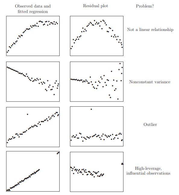
Figure: Residums Plots

Here’s a practical example using the built-in cars dataset in R, which contains data on car speeds and stopping distances. This example will walk you through scatter plots, box plots, density plots, and a bubble plot.

a. Scatter Plot with Best Fit Line

This scatter plot visualizes the relationship between car speed and stopping distance. The scatter.smooth() function will plot the data along with a smoothed line to help visualize the trend.

# Scatter plot with a smooth line
scatter.smooth(x = cars$speed, y = cars$dist, main = "Stopping Distance vs Speed",
               xlab = "Speed (mph)", ylab = "Stopping Distance (ft)")

b. Box Plot to Check for Outliers

Box plots help identify any outliers in the speed and distance variables.

# Set up the plot area to display two plots side by side
par(mfrow = c(1, 2))

# Box plot for speed
boxplot(cars$speed, main = "Box Plot for Speed", 
        sub = paste("Outliers:", paste(boxplot.stats(cars$speed)$out, collapse = ", ")))

# Box plot for distance
boxplot(cars$dist, main = "Box Plot for Distance", 
        sub = paste("Outliers:", paste(boxplot.stats(cars$dist)$out, collapse = ", ")))

c. Density Plot to Visualize Distribution

Density plots are useful for checking the distribution of variables. Here, we use the e1071 package to calculate skewness and visualize the density of speed and distance.

# Load the e1071 library to calculate skewness
library(e1071)

# Set up the plot area to display two plots side by side
par(mfrow = c(1, 2))

# Density plot for speed
plot(density(cars$speed), main = "Density Plot: Speed", xlab = "Speed", 
     ylab = "Density", sub = paste("Skewness:", round(skewness(cars$speed), 2)))
polygon(density(cars$speed), col = "blue", border = "black")

# Density plot for distance
plot(density(cars$dist), main = "Density Plot: Distance", xlab = "Distance", 
     ylab = "Density", sub = paste("Skewness:", round(skewness(cars$dist), 2)))
polygon(density(cars$dist), col = "blue", border = "black")

d. Bubble Plot to Add a Third Dimension

A bubble plot is a scatter plot where the size of the bubbles represents a third variable. Here, we use speed for bubble size to illustrate its relationship with distance.

# Bubble plot with bubble size representing speed
symbols(cars$speed, cars$dist, circles = cars$speed, inches = 0.5,
        main = "Bubble Plot: Distance vs Speed", xlab = "Speed (mph)", ylab = "Stopping Distance (ft)")

This code provides an initial analysis and visual overview of the relationships and distributions in the dataset, which can be valuable before applying further modeling or statistical techniques.

2. Normality

The residuals can be assessed for normality using a Q–Q plot

When the errors are not normal, least squares estimates may not be optimal. They will still be best linear unbiased estimates, but other robust estimators may be more effective. Also tests and confidence intervals are not exact. However, only long-tailed distributions cause large inaccuracies. Mild nonnormality can safely be ignored and the larger the sample size the less troublesome the nonnormality. For short-tailed distributions, the consequences of nonnormality are not serious and can reasonably

The Shapiro-Wilk test is a formal test for normality, The null hypothesis is that the the residuals are normal.:

shapiro.test (residuals (g))

3. Correlated Errors

Graphical checks include plots of \(\hat{\varepsilon}\) against time and \(\hat{\varepsilon}_{i}\) against \(\hat{\varepsilon}_{i-1}\) while the Durbin Watson test uses the statistic (The null distribution based on the assumption of uncorrelated errors follows a linear combination of \(\chi^{2}\) distributions.): \[ D W=\frac{\sum_{i=2}^{n}\left(\hat{\varepsilon}_{i}-\hat{\varepsilon}_{i-1}\right)^{2}}{\sum_{i=1}^{n} \hat{\varepsilon}_{i}^{2}} \]

2. Finding Unusual Observations

Studentized Residuals

The studentized residual \(r_i\) is given by: \[ r_{i} = \frac{\hat{\varepsilon}_{i}}{\hat{\sigma} \sqrt{1 - h_{i}}} \] where \(\hat{\varepsilon}_i\) is the residual for observation \(i\), \(\hat{\sigma}\) is the standard error of the residuals, and \(h_i\) is the leverage for observation \(i\).

If the model assumptions hold, the variance \(\operatorname{var}(r_i) = 1\), and the correlation \(\operatorname{corr}(r_i, r_j)\) tends to be small. Studentized residuals are often preferred in residual plots because they are standardized to have equal variance, correcting the natural non-constant variance of residuals under constant error variance assumptions. However, if heteroscedasticity is present, studentization alone cannot correct for it.

Outlier

An outlier is an observation that doesn’t fit the model well, often having a large residual. In linear regression, an outlier is defined as an observation whose value on the dependent variable is unusual given its predictor values. It may indicate a unique sample property or possibly a data entry error.

To identify outliers, compute: \[ \hat{y}_{(i)} = x_{i}^{T} \hat{\beta}_{(i)} \] where \(\hat{y}_{(i)}\) is the predicted value for observation \(i\) after excluding it from the model fit. If \(\hat{y}_{(i)} - y_i\) is large, then case \(i\) is considered an outlier. To quantify this, the variance of \(y_i - \hat{y}_{(i)}\) is given by: \[ \operatorname{var}\left(y_{i} - \hat{y}_{(i)}\right) = \hat{\sigma}_{(i)}^{2}\left(1 + x_{i}^{T}\left(X_{(i)}^{T} X_{(i)}\right)^{-1} x_{i}\right) \] We define jackknife residuals (or externally studentized residuals) as: \[ t_{i} = \frac{y_{i} - \hat{y}_{(i)}}{\hat{\sigma}_{(i)} \sqrt{1 + x_{i}^{T}\left(X_{(i)}^{T} X_{(i)}\right)^{-1} x_{i}}} \] which, under correct model assumptions, follows a \(t\)-distribution with \(n - p - 1\) degrees of freedom if \(\varepsilon \sim \mathrm{N}(0, \sigma^2 I)\). Alternatively, \(t_i\) can be computed as: \[ t_{i} = \frac{\hat{\varepsilon}_{i}}{\hat{\sigma}_{(i)} \sqrt{1 - h_{i}}} = r_{i}\left(\frac{n - p - 1}{n - p - r_{i}^{2}}\right)^{1 / 2} \] allowing us to avoid performing \(n\) separate regressions. Since \(t_i \sim t_{n - p - 1}\), we can use it to test if case \(i\) is an outlier.

Leverage

An observation has high leverage if its predictor values are far from the mean, meaning it can exert significant influence on the regression coefficients. The leverage value \(h_i = H_{ii}\) is useful for diagnostics. Since \[ \operatorname{var}(\hat{\varepsilon}_{i}) = \sigma^2 (1 - h_{i}), \] a high leverage \(h_i\) will reduce \(\operatorname{var}(\hat{\varepsilon}_{i})\), indicating that observation \(i\) has a significant influence on the model.

Influence

An observation is influential if its removal significantly changes the estimated regression coefficients. Influence is often seen as a product of leverage and residual size.

The Cook’s Distance is a popular diagnostic for influence, summarizing information into a single value for each observation: \[ D_{i} = \frac{(\hat{y} - \hat{y}_{(i)})^{T}(\hat{y} - \hat{y}_{(i)})}{p \hat{\sigma}^{2}} = \frac{1}{p} r_{i}^{2} \frac{h_{i}}{1 - h_{i}} \] where \(p\) is the number of predictors in the model, and \(r_i\) and \(h_i\) are the studentized residual and leverage for observation \(i\), respectively.

3. Checking the Structure of the Model

We can look at plots of \(\hat{\varepsilon}\) against \(\hat{y}\) and \(x_{i}\) to reveal problems or just simply look at plots of \(y\) against each \(x_{i} .\)

The disadvantage of these graphs is that other predictor variables affect the relationship. Partial regression or increased variable graph can help isolate the effect of \(x_{i}\) Look at the response that removes the expected effect of other \(X_s\): Partial regression (left) and partial residual (right) plots

\[ y-\sum_{j \neq i} x_{j} \hat{\beta}_{j}=\hat{y}+\hat{\varepsilon}-\sum_{j \neq i} x_{j} \hat{\beta}_{j}=x_{i} \hat{\beta}_{i}+\hat{\varepsilon} \]

Implementation

Implementation using SAS Proc Reg

Options

Here’s an overview of various options used in regression analysis and diagnostic plotting, along with their descriptions:

Options	Description
STB	Outputs the standardized partial regression coefficient matrix.
CORRB	Outputs the parameter estimation matrix.
COLLINOINT	Performs multicollinearity analysis on predictor variables.
P	Outputs individual observations, predicted values, and residuals.
R	Outputs each individual observation, residuals, and standard errors.
CLM	Outputs the 95% confidence interval limits for the mean of the dependent variable.
CLI	Outputs the 95% confidence interval limits for each predicted value.
MSE	Requests the variance of the random disturbance term to be output.
VIF	Outputs the Variance Inflation Factor (VIF), which measures multicollinearity. Higher VIF indicates greater variance due to multicollinearity.
TOL	Outputs the tolerance level for multicollinearity. A smaller TOL suggests that more of the variable’s variance is explained by other predictors, indicating potential multicollinearity.
DW	Outputs the Durbin-Watson statistic to check for autocorrelation.
Influence	Diagnoses outliers by outputting statistics for each observation. Cook’s D > 50% or defits/debetas > 2 suggests a significant influence of the point.

Plot Options

Plot Options	Description
FITPLOT	Scatter plot with regression line and confidence prediction bands.
RESIDUALS	Residuals of the independent variable.
DIAGNOSTICS	Diagnostic plots (includes the following plots).
COOKSD	Plot of Cook’s D statistic for influence diagnostics.
OBSERVEDBYPREDICTED	Plot of the observed dependent variable against predicted values.
QQPLOT	Q-Q plot to test for normality of residuals.
RESIDUALBYPREDICTED	Plot of residuals versus predicted values.
RESIDUALHISTOGRAM	Histogram of residuals.
RFPLOT	Residuals vs Fitted values plot.
RSTUDENTBYLEVERAGE	Plot of studentized residuals versus leverage.
RSTUDENTBYPREDICTED	Plot of studentized residuals versus predicted values.

These options and plots are valuable for evaluating model fit, diagnosing potential issues such as multicollinearity, identifying outliers, and checking assumptions like normality and homoscedasticity of residuals.

Diagnose

Hat matrix diagonal SAS

The hat matrix diagonal measure is used to identify unusual values of the explanatory variables. The hat matrix depends only on the explanatory values and not on the dependent y values. The interpretation, then, is that the hat matrix is a measure of leverage among the independent, explanatory variables only. In contrast, a plot of residuals identifies observations that are unusual in terms of their Y values that we wish to explain. The hat matrix diagonal measure is used to identify unusual values of the explanatory variables.

The “U” shape is a shape common to most hat matrix diagrams. We can think that the highest and lowest observed values of the explanatory variables are also the furthest away from the data center and will have the greatest impact. Observations close to the data center should have the least influence.

proc reg data=cold;
    model maxt = lat long alt / p r influence ;
    output out=inf h=h p=p r=r;
    run;
proc gplot data=inf;
    plot h * p;
run;

Jackknife Diagnostics SAS

The jackknife measures how much the fitted model changes when one observation is deleted and the model is refitted. If an observation is deleted from the data set, and the new fit is very different from the original model based on the complete data set, the observation is considered to have an impact on the fit

proc reg data=cold;
title2 ’Explain max Jan temperature’;
model maxt = lat long alt / p influence partial;
ods output OutputStatistics = diag;
run;
title2 ’Examine diagnostic data set’;
proc print data=diag;
run;

Partial Regression Plots SAS

One way to solve the problem of the individual contribution of each explanatory variable is to use partial correlation and partial regression plots. These are obtained using the /partial option in proc reg.

proc reg data=lowbw;
    model birthwt = headcirc length gestage momage toxemia
    / partial influence p r pcorr1 pcorr2;
    ods output OutputStatistics = diag;
run;

Implementation using R

Here’s a summary of commonly used functions in R for model diagnostics and checking assumptions, particularly useful when working with linear models (lm objects). These functions help evaluate model fit, detect heteroscedasticity, multicollinearity, and autocorrelation, and identify high leverage or influential points.

Title	Function
Predicted Values	fitted(bank.lm)
Model Coefficients	coef(bank.lm)
Residual Sum of Squares	deviance(bank.lm)
Residuals	residuals(bank.lm)
ANOVA Table	anova(bank.lm)
Confidence Interval	confint(bank.lm, level = 0.95)
Heteroscedasticity Test	library(car) then ncvTest(bank.lm)
Multicollinearity Check (VIF > 10)	vif(bank.lm)
Autocorrelation Test	durbinWatsonTest(bank.lm)
High Leverage Points (greater than 2–3 times mean)	hatvalues(bank.lm)
Influential Points	cooks.distance(bank.lm)
Outliers, High Leverage, and Influential Points	influence.measures(bank.lm)
Influence Plot	influencePlot(bank.lm)

These functions can be run on an lm model object (e.g., bank.lm) to examine various diagnostic aspects and validate model assumptions.

Model Selection

Statistical Measures to Assess Model Fit and Compare Models

These statistical measures are essential tools in regression analysis. They help determine the best model fit by balancing the complexity of the model (number of predictors) and its accuracy in predicting new data. RMSE and MSE are direct measures of residual errors, adjusted \(R^2\) provides a context-sensitive quality metric, Mallows’ \(C_p\) offers a method for model comparison, and AIC/BIC guide the selection of models based on their information loss with a focus on preventing overfitting.

1. Root Mean Square Error (RMSE) and Residual Sum of Squares (RSS):

• RMSE is defined as the square root of the average of squared residuals, computed as \(\text{RMSE} = \sqrt{\frac{\text{RSS}}{n-p}}\), where \(n\) is the number of observations and \(p\) is the number of explanatory variables (including the intercept).
• RSS is the sum of the squares of residuals, reflecting the total squared deviation of predicted values from observed values.

2. Mean Square Error (MSE):

• MSE measures the average of the squares of the errors, essentially quantifying the quality of an estimator in reproducing the observed values.
• It is calculated by dividing RSS by the degrees of freedom, \((n-p)\), giving \(\text{MSE} = \frac{\text{RSS}}{n-p}\).

3. Adjusted R-Squared (Adjusted \(R^2\)):

• This statistic adjusts the R-squared value to account for the number of predictors in a model, providing a measure that penalizes excessive use of predictors.
• It is calculated as: \[ \text{adj} R^2 = 1 - \left(1-R^2\right)\frac{n-1}{n-p} \]
• Adjusted \(R^2\) compares the explanatory power of regression models that contain different numbers of predictors.

4. Mallows’ C_p:

• Introduced by Colin Mallows in 1964, this criterion is used to assess the quality of regression models based on their predictive accuracy.
• It is defined as: \[ C_p = \frac{\text{RSS}}{s^2} + 2p - n \]
• Mallows’ \(C_p\) aims to identify models with the correct number of predictors, where a good model has a \(C_p\) roughly equal to \(p\) (the number of predictors).

5. Akaike Information Criterion (AIC) and Bayesian Information Criterion (BIC):

• AIC and BIC are used to evaluate model fit with a penalty for the number of parameters, helping to avoid overfitting.
• AIC is calculated as: \[ \text{AIC} = n \ln\left(\frac{\text{RSS}}{n}\right) + 2p \]
• BIC is calculated as: \[ \text{BIC} = n \ln\left(\frac{\text{RSS}}{n}\right) + p \ln(n) \]
• Both criteria are based on the likelihood of the data under the model, with BIC adding a stronger penalty for the number of parameters than AIC.

Here’s an overview of three popular model selection methods in regression analysis: forward stepwise selection, backward stepwise regression, and best subset regression. Each approach can be used to choose the most appropriate predictors in a model.

Model Comparasion

Model comparison in linear regression involves statistically evaluating whether one model provides a significantly better fit to the data than another. This comparison is crucial when determining the most appropriate set of predictors, assessing model complexity, or validating theoretical expectations against empirical data. Several techniques are commonly used for this purpose, including F-tests for nested models, adjusted R-squared, Akaike Information Criterion (AIC), and Bayesian Information Criterion (BIC).

1. F-test for Nested Models

The F-test is used to compare models where one model is a special case of the other (i.e., a nested model). The test evaluates whether the more complex model (with more predictors) significantly improves the fit of the model compared to the simpler model.

• Null Hypothesis (H0): The simpler model is sufficient, and the additional predictors in the complex model do not significantly improve the fit.
• Alternative Hypothesis (H1): The complex model provides a significantly better fit to the data.

The F-statistic is calculated as: \[ F = \frac{(\text{RSS}_{\text{simple}} - \text{RSS}_{\text{complex}}) / (p_{\text{complex}} - p_{\text{simple}})}{\text{RSS}_{\text{complex}} / (n - p_{\text{complex}})} \] Where: - \(\text{RSS}_{\text{simple}}\) and \(\text{RSS}_{\text{complex}}\) are the residual sums of squares from the simpler and more complex models, respectively. - \(p_{\text{simple}}\) and \(p_{\text{complex}}\) are the number of parameters in the simpler and more complex models. - \(n\) is the number of observations.

If the calculated F-value exceeds the critical value from the F-distribution for a given significance level (usually 0.05), the null hypothesis is rejected, indicating that the more complex model provides a better fit.

2. Adjusted R-squared

Adjusted R-squared is used to compare models with different numbers of predictors. Unlike R-squared, which always increases as more predictors are added, adjusted R-squared penalizes for the number of predictors in the model, providing a more accurate measure of model performance.

• A higher adjusted R-squared value indicates a better model, provided the increase is significant.

3. Information Criteria: AIC and BIC

Both AIC and BIC provide a means of model comparison by balancing goodness of fit with model complexity: - AIC (Akaike Information Criterion): \[ \text{AIC} = 2k - 2\ln(L) \] Where \(k\) is the number of parameters and \(L\) is the likelihood of the model.

• BIC (Bayesian Information Criterion): \[ \text{BIC} = k\ln(n) - 2\ln(L) \] Where \(n\) is the number of observations.

For both criteria, a lower value indicates a better model. BIC typically imposes a heavier penalty for the number of parameters than AIC, making it more stringent against complex models.

4. Analysis of Variance (ANOVA)

ANOVA can be used to compare models by examining the variance explained by each model. It’s particularly useful for comparing models that are not nested.

• The ANOVA table will show whether the addition of variables significantly increases the explained variance, indicating a better model.

g2 < - 1m (sr ˜ pop75 + dpi + ddpi, savings)

## d compute the RSS and the F-statistic:
(rss2 < - deviance (g2))
(fstat < - (deviance (g2)-deviance (g))/(deviance (g)/df.residual(g)))
## P value
1-pf (fstat, l, df.residual(g))

## relate this to the t-based test and p-value by:
sqrt (fstat) 
(tstat < - summary(g)$coef[2, 3])
2 * (l-pt (sqrt (fstat), 45))

## more convenient way to compare two nested models is:
anova (g2, g)

## Analysis of Variance Table
## Model 1: sr ˜ pop75 + dpi + ddpi
## Model 2: sr ˜ pop15 + pop75 + dpi + ddpi

Four Method

1. Forward Stepwise Selection

Forward selection is a stepwise approach in regression analysis where predictors are added one at a time into the model, and at each step, the variable that provides the most statistically significant improvement to the model is included. This method is particularly useful when dealing with a large number of variables, as it helps in identifying a potentially optimal subset of predictors that contribute meaningfully to predicting the response variable.

Process: 1. Initiation: Begin with a model that includes no predictors. This means starting from a baseline model where only the intercept is considered.

2. Selection of Predictors: At each step, each variable not yet in the model is considered for addition. The selection criterion for each potential new variable is based on the F-statistic, where the variable with the maximum F-statistic that exceeds a certain threshold is added to the model.

3. Criteria for Adding Variables: The variable to be added is chosen based on its ability to maximize the F-statistic among all variables not already in the model. The F-statistic here measures how much a variable improves the model fit by comparing the change in residual sum of squares before and after the inclusion of the variable.

4. Stop Condition: This process continues until adding a new variable does not significantly improve the model anymore, based on the F-statistic. Typically, a pre-defined significance level (such as 0.05) is used as a cutoff. If the highest F-statistic among the remaining variables does not meet this threshold, the process stops.

5. Final Model: The result is a model that includes a subset of variables that have been systematically chosen to optimize the model’s predictive accuracy and explanatory power, based on the criterion of the F-statistic.

Advantages and Limitations: - Advantage: Forward selection is computationally efficient and can be particularly useful when the number of observations is much greater than the number of variables. It allows for the building of parsimonious models that avoid overfitting by limiting the number of predictors.

• Limitation: One major limitation of this method is its potential to overlook the effects of combining variables. Since it evaluates variables sequentially rather than in combination, interactions or combined effects that might be significant could be missed. Moreover, this method is greedy; once a variable is included, it is never removed, which might lead to suboptimal models if a variable becomes redundant after additional variables are added.

Example Code in SAS:

title2 'Forward stepwise selection';
proc reg;
    model birthwt = headcirc length gestage momage toxemia / selection=f;
run;

2. Backward Stepwise Regression

Backward elimination is a stepwise regression technique that starts with a full model, including all potential predictors, and systematically removes the least significant predictors one by one to simplify the model while attempting to maintain its explanatory power. This method is especially useful when you have a large number of predictors and are looking to identify a more parsimonious model that still effectively captures the relationships in the data.

Process:

1. Start with a Full Model: Initiate the process with a full model that includes all candidate predictors.

2. Evaluate and Remove: At each step, evaluate the statistical significance of the predictors. The predictor with the highest p-value (least significant) is removed from the model, provided its p-value exceeds a pre-specified significance level (often set at 0.05).

3. Iterate: Repeat the process of removing the least significant predictor until all remaining predictors have a p-value below the threshold, indicating that they are statistically significant contributors to the model.

4. Stopping Criterion: The process stops when removing any further predictors would lead to a model where all remaining variables are statistically significant, or when removing additional predictors significantly worsens the model according to a specific criterion (e.g., a substantial decrease in R-squared or increase in AIC/BIC).

Advantages and Limitations:

• Advantages:
  • Provides an automated approach to model simplification, which can be invaluable in scenarios with large datasets.
  • Helps in focusing on the most significant predictors, reducing the complexity and potentially enhancing the interpretability of the model.
• Limitations:
  • The choice of significance level for removal can impact the final model. Setting this threshold too low might retain unnecessary predictors, while setting it too high might exclude important ones.
  • It can lead to suboptimal models if the removed variables have significant interaction effects with the variables left in the model.
  • It does not account for the possibility that a predictor insignificant in a full model may become significant when non-informative predictors are removed.

Example Code in SAS:

proc reg;
    model birthwt = headcirc length gestage momage toxemia / selection=b;
run;

3. Stepwise Selection Method

Overview: Stepwise selection is a systematic procedure for adding and removing predictors based on their statistical significance in a regression model. It is a popular approach due to its ability to handle large datasets with many variables, refining the model to include only those variables that have a significant impact on the dependent variable.

Process:

1. Starting Point: The stepwise procedure can start with no variables in the model and then add them sequentially (similar to forward selection), or it can start with all potential predictors in the model and remove them one by one (akin to backward elimination).

2. Forward Step:

   • Variables are added one at a time based on a specified criterion, typically the F-statistic.
   • Each potential new variable is assessed to determine whether its inclusion significantly improves the model fit.
   • If adding the variable substantially improves the model (based on a predetermined threshold like a p-value or an increase in R-squared), it is included in the model.

3. Backward Step:

   • After adding variables, the model is then assessed to see if all variables still contribute significantly.
   • Variables that do not meet the significance criterion are considered for removal.
   • This involves testing each variable in the model to see if removing it significantly worsens the model fit. If not, the variable is removed.

4. Criteria for Adding and Removing Variables:

   • The decision to add or remove a variable is based on specific criteria such as the p-value, with common thresholds being 0.05 for inclusion and 0.10 for removal.
   • The process continues iteratively, with variables being added or removed, refining the model progressively until no further variables meet the criteria for entry or removal.

Evaluation and Iteration:

• The method evaluates at each step whether any variables previously removed could now be significant and should be re-introduced, making the process dynamic and iterative.
• This iteration continues until adding or removing any more variables does not improve the model significantly.

Advantages and Limitations:

• Advantages: Stepwise selection can be more efficient than manually testing all possible combinations of variables, especially in datasets with a large number of variables. It helps in identifying a model that is simpler and still explains the data adequately.
• Limitations: This method can lead to models that are dependent on the order of the variables entered and might include variables that are marginally significant. It also tends to capitalize on chance correlations in the sample data, which may not generalize well to other datasets. The method can also overlook interaction effects unless explicitly included.

4. Best Subset Regression

Best Subset Regression is a method used in statistical modeling, specifically in regression analysis, to select a subset of predictors that provide the best fit to the model according to a specified criterion. This technique is considered exhaustive as it evaluates all possible combinations of predictors to identify the model that best explains the outcome variable.

Best subset regression is often used when there are a moderate number of predictors, and the analyst wants to determine which combination of variables predicts the outcome most effectively. Unlike stepwise selection methods that incrementally add or remove variables based on statistical tests, best subset regression reviews all potential models that can be created from the predictor set.

Best subset regression is particularly useful in situations where:

• The dataset is not excessively large.
• The number of predictors is moderate but the analyst wishes to ensure that all potential interactions and effects are considered.
• There is a need to rigorously test which predictors are most important for predicting the outcome.

Process

1. Generate All Possible Models:
   • For each possible combination of the predictor variables, a separate model is fit. For example, if there are three predictors, this method would evaluate all possible models: each predictor alone, each pair of predictors, and the model containing all three predictors.
2. Evaluate Model Fit:
   • Each model is assessed based on a predetermined statistical criterion, commonly the Akaike Information Criterion (AIC), Bayesian Information Criterion (BIC), adjusted R-squared, or Mallows’ Cp. These criteria balance model fit with complexity to prevent overfitting.
3. Select the Best Model:
   • The model with the best value (lowest for AIC/BIC, highest for adjusted R-squared) is selected as the optimal model. This step involves comparing the performance of potentially many models.

Advantages and Limitations

• Advantages:
  • Comprehensiveness: By considering every possible combination of variables, best subset regression can be very thorough, making it less likely to miss combinations that provide a good fit.
  • Flexibility: It allows the analyst to review and choose from models based on various criteria, tailoring the selection to the specific needs of the analysis.
• Limitations:
  • Scalability: The number of potential models increases exponentially with the number of predictors, making this method computationally expensive and practically infeasible for large datasets.
  • Risk of Overfitting: Despite using criteria that penalize model complexity, there’s still a risk of overfitting, especially when the number of predictors is large relative to the sample size.

Example Code in SAS:

title2 'Selecting the best of all possible regression models';
proc reg;
    model birthwt = headcirc length gestage momage toxemia / selection=cp adjrsq r best=5;
run;

The / selection = cp adjrsq r option directs SAS to use Mallow’s \(C_p\) criterion to rank models, displaying both adjusted and unadjusted R-squared statistics. best=5 specifies that SAS should display the top 5 models.

Example Code in R:

# Load necessary libraries
library(leaps) 
library(alr3)

# Load data
data(water)
socal.water <- water[ ,-1]  # Remove the first column if not needed

# Fit the full model
fit <- lm(BSAAM ~ ., data = socal.water)
summary(fit)

# Perform best subset regression
sub.fit <- regsubsets(BSAAM ~ ., data = socal.water)
best.summary <- summary(sub.fit)
print(best.summary)

# Identifying models with minimum or maximum values
which.min(best.summary$rss)   # Minimum RSS
which.min(best.summary$bic)   # Minimum BIC
which.max(best.summary$adjr2) # Maximum Adjusted R-squared

# Plot model evaluation
par(mfrow = c(1, 2))
plot(best.summary$cp, xlab = "Number of features", ylab = "Cp")
plot(sub.fit, scale = "Cp")

This R code performs best subset regression on the water dataset. The regsubsets() function from the leaps package evaluates all possible subsets, and the summary() provides metrics like RSS, BIC, and adjusted R-squared, which you can use to choose the best model. The which.min() and which.max() functions help identify the subset with the best criterion value.

k-Fold Cross-Validation

Background:

Professor Tappi from Wright State University highlights the importance of testing regression models rigorously for predicting future observations. When a model is trained and tested on the same dataset, it can lead to overly optimistic conclusions about the model’s predictive performance, as it may not generalize well to new data. For a more unbiased assessment of prediction accuracy, a common approach is to hold back one observation, fit the model on the remaining data, and then use the held-out observation to test the prediction. This leave-one-out method reduces bias in evaluating model performance.

Purpose of k-Fold Cross-Validation:

While splitting the data into training and test sets (e.g., 80/20 split) might provide an initial performance estimate, it doesn’t guarantee consistent results on other subsets. k-Fold Cross-Validation provides a more robust test by building multiple models on different portions of the data, ensuring the model’s performance is not overly dependent on one specific train-test split.

Procedure for k-Fold Cross-Validation:

1. Divide the data into k mutually exclusive, random portions.
2. Use each portion as a test set while training the model on the remaining k-1 portions.
3. Calculate the mean squared error (MSE) for each fold.
4. Average the MSEs across all k folds to obtain a cross-validated error estimate.

This cross-validated error estimate can then be used to compare models and helps determine which model generalizes best to new data.

Skewness

Basic Transformations for Skewed Data

Transformations can be applied to data to address skewness and better meet model assumptions, particularly when dealing with positively or negatively skewed distributions. Here are some commonly used transformations:

1. Square-Root Transformation (for moderate skew):

   • For positively skewed data: \(\sqrt{x}\)
   • For negatively skewed data: \(\sqrt{\text{max}(x + 1) - x}\)

2. Log Transformation (for greater skew):

   • For positively skewed data: \(\log_{10}(x)\)
   • For negatively skewed data: \(\log_{10}(\text{max}(x + 1) - x)\)

   The logarithmic transformation pulls in large values and spreads out smaller values, reducing the impact of outliers.

3. Inverse Transformation (for severe skew):

   • For positively skewed data: \(\frac{1}{x}\)
   • For negatively skewed data: \(\frac{1}{\text{max}(x + 1) - x}\)

**Attention*

When data does not meet the normality assumption, consider running statistical tests (e.g., t-tests or ANOVA) on both transformed and untransformed data to assess if there are significant differences in results. If both tests lead to the same conclusion, you may opt to avoid transformation and proceed with the original data for simplicity.

Be aware that transformations can complicate analysis. For instance, after transforming data and running a t-test, the results indicate differences based on the transformed scale (e.g., log scale), making interpretation less straightforward. Therefore, transformations are usually avoided unless necessary for valid analysis.

---

Additional Approaches for Skewed Data

If the response variable \(y\) is continuous, positive, and has a right-skewed histogram (long right tail), consider these modeling options:

1. Box-Cox Transformation: This technique identifies an optimal power transformation to stabilize variance and make the data more normally distributed.
2. Gamma Regression: A gamma distribution can model response variables with positive values and right skew, offering a more flexible alternative to transformations for highly skewed data.

Transforming the Response Variable \(y\) for Normality

To make the density of a right-skewed response variable \(y\) more normal, we can apply a transformation based on a parameter \(\lambda\), which is optimized via maximum likelihood estimation.

The transformation is given by: \[ \tilde{y} = \begin{cases} \frac{y^{\lambda} - 1}{\lambda}, & \text{if } \lambda \neq 0 \\ \ln y, & \text{if } \lambda = 0 \end{cases} \]

Choosing the Optimal Value of \(\lambda\)

The best \(\lambda\) is chosen by fitting a linear model on transformed \(y\) values across discrete \(\lambda\) values and selecting the \(\lambda\) that maximizes the likelihood function. However, since real-world data may not follow an exact normal distribution, researchers often “round” \(\lambda\) to produce interpretable transformations.

The table below summarizes suggested transformations based on the range of optimal \(\lambda\):

Here’s the table in Markdown format:

Range for Optimal \(\lambda\)	Recommended \(\lambda\)	Transformed \(\tilde{y}\)	Transformation Name
[-2.5, -1.5)	-2	\(\frac{1}{2} \left( 1 - \frac{1}{y^2} \right)\)	Inverse Square
[-1.5, -0.75)	-1	\(1 - \frac{1}{y}\)	Inverse (Reciprocal)
[-0.75, -0.25)	-0.5	\(2 \left( 1 - \frac{1}{\sqrt{y}} \right)\)	Inverse Square Root
[-0.25, 0.25)	0	\(\ln y\)	Natural Logarithm
[0.25, 0.75)	0.5	\(2 (\sqrt{y} - 1)\)	Square Root
[0.75, 1.5)	1	\(y - 1\)	Linear
[1.5, 2.5]	2	\(\frac{1}{2} (y^2 - 1)\)	Square

The fitted model for the transformed response \(\tilde{y}\) can be represented as: \[ \widehat{\mathbb{E}}(\tilde{y}) = \widehat{\mathbb{E}}\left(\frac{y^{\lambda} - 1}{\lambda}\right) = \widehat{\beta}_{0} + \widehat{\beta}_{1} x_{1} + \cdots + \widehat{\beta}_{k} x_{k} \]

*Interpretation of Estimated Regression Coefficients**

• For a continuous predictor \(x_{1}\), the estimated coefficient \(\widehat{\beta}_{1}\) represents the change in the mean of the transformed response \(\widehat{\mathbb{E}}(\tilde{y})\) for a one-unit increase in \(x_{1}\), assuming other predictors remain constant.
• If \(x_{1}\) is an indicator variable, \(\widehat{\beta}_{1}\) represents the difference in the mean of the transformed response \(\widehat{\mathbb{E}}(\tilde{y})\) between \(x_{1} = 1\) and \(x_{1} = 0\), with other predictors unchanged.

Interaction Analysis

Simple Slopes Analysis

If an interaction term is significant, a simple slopes analysis is needed.

Simple slopes analysis is used to interpret the interaction effects in a regression model. When an interaction term is included, the regression output shows the slope of the predictor when the moderator variable is at zero—often an arbitrary or theoretically irrelevant value. To better understand the nature of the interaction, simple slopes analysis examines how the effect of one predictor on the dependent variable varies at different levels of the moderator.

Since the moderator is often continuous, we typically select three representative values to represent its low, average, and high levels: \[ M_{a} - SD_{a}, \quad M_{a}, \quad M_{a} + SD_{a} \] where \(M_{a}\) is the mean and \(SD_{a}\) is the standard deviation of the moderator \(a\).

For example, in the model: \[ y = b_{0} + b_{1}x + b_{2}a + b_{3}(x - M_{x})(a - M_{a}), \] the regression output provides slopes for \(x\) at the mean of \(a\). However, we cannot obtain statistical metrics (e.g., significance tests, confidence intervals) for slopes at different levels of \(a\) directly from this output.

Steps for Simple Slopes Analysis

To calculate simple slopes at different levels of \(a\), we adjust the moderator \(a\) by subtracting values (e.g., \(\Delta\)) to generate three new interaction terms: \[ \text{int}' = (x - M_{x}) \cdot (a - \Delta), \] where each new interaction term corresponds to a different level of \(a\): 1. When \(\Delta = M_{a}\): The regression equation remains the same as the original, with \(B_{1} = b_{1}\). 2. When \(\Delta = M_{a} - SD_{a}\): \(B_{1} = b_{1} - b_{3} \cdot SD_{a}\). 3. When \(\Delta = M_{a} + SD_{a}\): \(B_{1} = b_{1} + b_{3} \cdot SD_{a}\).

By running three regressions with these new interaction terms, we obtain the regression coefficients for \(x\), which represent the simple slopes at different levels of \(a\). The statistical indicators for \(B_{1}\) (significance, confidence intervals, standardized coefficients, etc.) are provided in each regression output.

Automating Simple Slopes Analysis with sim_slopes

The sim_slopes function automates this process by taking a regression model with an interaction term as input and performing simple slopes analysis, yielding statistical information for each slope at the specified levels of the moderator.

Plotting Interactions with Continuous Predictors in Regression Models

Here’s an example of how to plot interaction effects in regression models using the interactions package in R.

Interactions of Continuous Variables

library(jtools) # for summ()
library(interactions) # for interact_plot()

# Using the `state.x77` dataset
states <- as.data.frame(state.x77)
fiti <- lm(Income ~ Illiteracy * Murder + `HS Grad`, data = states)
summ(fiti)

# Basic interaction plot
interact_plot(fiti, pred = Illiteracy, modx = Murder)

# Customizing labels and colors
interact_plot(fiti, pred = Illiteracy, modx = Murder,
              x.label = "Custom X Label", y.label = "Custom Y Label",
              main.title = "Sample Plot", legend.main = "Custom Legend Title",
              colors = "seagreen")

Interactions Involving Factors

# Using the `iris` dataset
fitiris <- lm(Petal.Length ~ Petal.Width * Species, data = iris)
interact_plot(fitiris, pred = Petal.Width, modx = Species)

# Plot only specific levels of a factor
interact_plot(fitiris, pred = Petal.Width, modx = Species,
              modx.values = c("versicolor", "virginica"))

Adding Observed Data Points to Interaction Plots

# Continuous interaction with observed points
interact_plot(fiti, pred = Illiteracy, modx = Murder, plot.points = TRUE)

# Categorical interaction with observed points and jitter
interact_plot(fitiris, pred = Petal.Width, modx = Species,
              plot.points = TRUE, jitter = 0.1, point.shape = TRUE)

Confidence Bands

# Adding confidence intervals with robust standard errors
interact_plot(fiti, pred = Illiteracy, modx = Murder, interval = TRUE, int.width = 0.8)

Checking Linearity Assumption

Testing the linearity assumption ensures that the relationship between the predictor and response variables is linear for different levels of the moderator. If the relationship is nonlinear, the interaction plot will show a “bend.”

# Generate synthetic data to illustrate linearity check
set.seed(99)
x <- rnorm(n = 200, mean = 3, sd = 1)
err <- rnorm(n = 200, mean = 0, sd = 4)
w <- rbinom(n = 200, size = 1, prob = 0.5)

# Example where linearity assumption is satisfied
y_1 <- 5 - 4*x - 9*w + 3*w*x + err
model_1 <- lm(y_1 ~ x * w)
summ(model_1)
interact_plot(model_1, pred = x, modx = w, linearity.check = TRUE, plot.points = TRUE)

# Example where linearity assumption is violated
x_2 <- runif(n = 200, min = -3, max = 3)
y_2 <- 2.5 - x_2^2 - 5*w + 2*w*(x_2^2) + err
data_2 <- as.data.frame(cbind(x_2, y_2, w))

model_2 <- lm(y_2 ~ x_2 * w, data = data_2)
summ(model_2)
interact_plot(model_2, pred = x_2, modx = w, linearity.check = TRUE, plot.points = TRUE)

# Polynomial fitting for non-linearity
model_3 <- lm(y_2 ~ poly(x_2, 2) * w, data = data_2)
summ(model_3)
interact_plot(model_3, pred = x_2, modx = w, data = data_2, linearity.check = TRUE, plot.points = TRUE)

These examples illustrate various ways to use interact_plot for visualizing interaction effects, adding data points, adjusting labels, and checking the linearity assumption.

Multicollinearity and Heteroskedasticity

Introduction

Multicollinearity occurs when two or more predictor variables in a multiple regression model are highly correlated, leading to instability in the estimation of the regression coefficients. This instability can increase the variance of the coefficient estimates and make the model sensitive to changes in the model, such as which variables are included or excluded from the model.

When some predictors are linear combinations of others, the matrix \(X^{T} X\) becomes singular, leading to exact collinearity. In this case, there is no unique least squares estimate of \(\beta\). If \(X^{T} X\) is nearly singular, this results in collinearity (often called multicollinearity), which can cause serious issues with estimating \(\beta\), interpreting the model, and assessing associated quantities.

• Multicollinearity does not reduce the predictive power or reliability of the model as a whole, nor does it affect the model’s ability to fit the data (i.e., it doesn’t affect the goodness of fit).
• However, it makes it difficult to assess the individual effect of each predictor on the dependent variable because it increases the standard errors of the coefficients. This can lead to coefficients being statistically insignificant when they should be significant.
• Due to the high correlation among predictors, it becomes challenging to pinpoint the exact contribution of each predictor to the outcome variable.
• It can also result in overestimating the importance of one variable while underestimating the importance of others, or it can cause the signs of coefficients to be counterintuitive (e.g., positive instead of negative and vice versa).

Diagnosis and Solutions:

• Multicollinearity can be diagnosed through various statistical methods such as examining the correlation matrix of the predictors, Variance Inflation Factor (VIF), and Tolerance.
• To address multicollinearity, one might consider removing or combining highly correlated variables, applying principal component analysis, or increasing the sample size to help stabilize the estimates.

In practical terms, if you suspect multicollinearity in your regression model, you should:

• Check correlation matrices and calculate VIF scores for the predictors. A VIF exceeding 5 (some suggest 10 as a threshold) is typically considered an indication of significant multicollinearity.
• Consider using regularization techniques like Ridge or Lasso, which can help in mitigating the impact of multicollinearity by penalizing large coefficients.

Impact on Linear Regression

Multicollinearity in linear regression occurs when two or more predictor variables are highly correlated, meaning they contain similar information about the variance in the dependent variable. This phenomenon can significantly affect the accuracy and interpretability of the regression analysis.

Effects of Multicollinearity on Linear Regression:

1. Coefficient Estimation:
   • Instability: Multicollinearity makes the coefficient estimates unstable. Small changes in the model or the data can lead to large variations in the coefficients. This instability can result in significant challenges when interpreting the results, as the coefficients may not accurately reflect the relationship between the predictors and the outcome.
   • Inflated Variances: The presence of multicollinearity increases the variances of the coefficient estimates. High variances result in wider confidence intervals and less reliable coefficient estimates, making it difficult to ascertain the true effect of each predictor.
2. Statistical Significance:
   • Reduced Precision: Due to the inflated variances, the standard errors of the coefficient estimates are also increased. This leads to a decrease in the t-statistic for each predictor, which can mask the true statistical significance of predictors. Important variables might appear statistically insignificant, leading to their exclusion from the model.
3. Model Interpretation:
   • Ambiguity in Results: With high multicollinearity, the coefficient for a predictor variable can be misleading. For instance, the sign of the coefficient might be opposite to what is expected intuitively, or it might suggest a larger or smaller effect than actually exists. This ambiguity complicates the interpretation and decision-making processes based on the model’s outputs.
4. Predictive Accuracy:
   • While multicollinearity affects the coefficients and their interpretation, it does not reduce the predictive accuracy of the model as a whole. If the goal is solely prediction, multicollinearity may not pose a serious issue. However, if the objective is to understand the influence of individual predictors, multicollinearity can significantly impair the clarity of these insights.

Detecting Normality, Independence, and Equality of Variance of Residuals

1. Normality of Residuals

• Assumption: The residuals \(e_i\) from the regression model are normally distributed. This assumption is crucial for the validity of inferential statistics related to the regression, such as hypothesis tests and confidence intervals for the coefficients.
• Implication: If the residuals are normally distributed, it implies that the estimates of the coefficients obtained through ordinary least squares (OLS) are the most efficient (smallest variance among unbiased estimators), and the statistical inference derived from these estimates (like t-tests for coefficients) will be valid.

2. Independence of Residuals

• Assumption: The residuals are independent of each other, which means that the value of one residual should not predict the value of another.
• Implication: Independence is key to preventing autocorrelation, particularly in time series data where the assumption can often be violated. When residuals are not independent, it can lead to misleadingly high or low estimates of the regression coefficients, affecting the reliability of the model’s predictions.

3. Homoscedasticity (Equal Variance of Residuals)

• Assumption: The variance of the residuals is constant across all levels of the independent variables. This assumption, called homoscedasticity, opposes the presence of heteroscedasticity, where the variance of residuals varies at different levels of the predictors.
• Implication: When residuals exhibit constant variance, it ensures that the regression model provides equal weight to all observations. If heteroscedasticity is present (i.e., the variance of residuals increases or decreases with the predicted values), it can lead to inefficiency in the estimates and affect the standard errors, which in turn can mislead conclusions about the significance of predictors.

Statistical Tests and Diagnostics

• To check these assumptions, various diagnostic tools and plots are used:
  • Normality: Histograms of residuals or Q-Q (quantile-quantile) plots can help visualize if residuals follow a normal distribution.
  • Independence: Autocorrelation functions (ACF) or plots of residuals against time can detect patterns that would suggest non-independence.
  • Homoscedasticity: Plots of residuals against predicted values or independent variables can be used to observe whether the spread of residuals remains constant across the range of predictions.

Addressing Violations

• If normality is violated: Transformations such as log, square root, or Box-Cox transformations can be applied to the response variable.
• If independence is violated: Adding lag variables or using time series analysis techniques might be necessary.
• If homoscedasticity is violated: Using robust standard errors or transforming the dependent variable can help mitigate this issue.

Detecting and Addressing Multicollinearity

There are several ways to detect collinearity:

1. Correlation Matrix: Examining the correlation matrix of predictors can reveal high pairwise correlations, which may indicate multicollinearity.

2. Regression of Each Predictor: Regress each predictor \(x_i\) on all other predictors and compute \(R_i^2\). Repeat for all predictors. An \(R_i^2\) close to 1 suggests issues, as it indicates a strong linear relationship with other predictors.

3. Eigenvalues of \(X^{T} X\): Compute the eigenvalues of \(X^{T} X\), where \(\lambda_1\) is the largest eigenvalue and others decrease. Small eigenvalues signal potential collinearity problems.

Solutions: To mitigate the effects of multicollinearity, analysts might consider:

• Removing Highly Correlated Predictors: If two variables convey similar information, consider removing one of them.
• Combining Predictors: Creating a new variable that combines the information of highly correlated variables can reduce multicollinearity.
• Principal Component Analysis (PCA): PCA can be used to transform the predictors into a set of orthogonal (uncorrelated) components, which can then be used in regression without the problems of multicollinearity.

Variance Inflation Factor (VIF)

Definition and Calculation: The Variance Inflation Factor (VIF) is a statistical measure that quantifies the extent of correlation and multicollinearity between independent variables in a regression analysis. High VIF values indicate high levels of multicollinearity, which can undermine the statistical significance of an independent variable and destabilize the regression coefficients.

The VIF for each variable is calculated using the following formula:

\[ \text{VIF}_j = \frac{1}{1 - R_j^2} \]

• \(R_j^2\) is the coefficient of determination from a regression of independent variable \(j\) on all the other independent variables.

Process:

1. Determine \(R_j^2\): For each independent variable in the model, regress this variable against all other independent variables and calculate the \(R^2\) value, which represents how well the other independent variables can predict this variable.

2. Calculate VIF: Use the \(R^2\) value obtained to calculate the VIF according to the formula provided. A VIF value greater than 1 indicates some level of multicollinearity, with higher values indicating higher multicollinearity.

Interpretation:

• Thresholds for VIF: Typically, a VIF value greater than 10 is considered indicative of significant multicollinearity, suggesting that the variable is highly collinear with at least one other variable. This threshold is used as a rule of thumb to diagnose problematic levels of multicollinearity.
• Impact of High VIF: High VIF values can lead to inflated variances for the coefficient estimates, which increases the standard errors and makes it difficult to determine the true effect of independent variables. This can result in unstable estimates of coefficients and misleading statistical tests.

Eigenvalues Criterion Method

The Eigenvalue Criterion method, also known as the Eigenvalue Decomposition method, is a sophisticated technique used to detect multicollinearity in multiple regression analyses. This method involves analyzing the eigenvalues of the correlation or covariance matrix derived from the predictor variables.

Step 1: Construct the Correlation or Covariance Matrix

Start by creating a correlation or covariance matrix for all predictor variables in your regression model. The choice between using a correlation matrix or a covariance matrix generally depends on the scaling of the variables; a correlation matrix, which standardizes variables, is often preferred because it allows for comparison on the same scale.

Step 2: Compute Eigenvalues

Calculate the eigenvalues of the matrix constructed in Step 1. Eigenvalues are calculated from the determinant equation of the matrix, which involves solving for roots where the determinant of (Matrix - Eigenvalue * Identity matrix) equals zero. This step can typically be executed using statistical software or packages that support linear algebra operations, such as R, Python (NumPy or SciPy), or MATLAB.

Step 3: Analyze the Eigenvalues

Examine the eigenvalues obtained from the computation:

• Zero or Near-Zero Eigenvalues: The presence of zero or very small eigenvalues indicates strong multicollinearity. This is because a zero eigenvalue suggests that the matrix is singular, implying that at least one variable is a perfect linear combination of others.
• Small Eigenvalues Relative to Others: If some eigenvalues are significantly smaller than others (but not zero), it suggests that there are near-linear dependencies among some of the variables.

Step 4: Consider the Condition Index

For a more detailed analysis, compute the Condition Index for the matrix, which is defined as the square root of the ratio of the maximum eigenvalue to each respective eigenvalue. A Condition Index: - Above 30 typically indicates a multicollinearity problem. - Values between 10 and 30 suggest moderate multicollinearity. - Values below 10 generally imply that multicollinearity is not a concern.

Step 5: Investigate Problematic Variables

If high multicollinearity is detected (through zero or small eigenvalues or high condition indices), further investigate to identify which variables are causing the issue. This might involve: - Looking at the eigenvectors corresponding to small eigenvalues, which can help identify which variables are contributing to multicollinearity. - Performing sensitivity analysis by sequentially removing variables and observing the effect on eigenvalues.

Step 6: Remedial Measures

Depending on the findings, consider taking remedial actions such as: - Removing one or more of the highly collinear variables. - Combining variables to reduce dimensionality. - Using regularization techniques such as Ridge or Lasso, which can help in handling multicollinearity by penalizing large coefficients.

Alternative with OLS

The standard assumptions for the error term \(\varepsilon\) are that it is independent and identically distributed (i.i.d.) with variance \(\sigma^2 I\) and that it follows a normal distribution for standard statistical inference. However, these assumptions are often violated, so we need alternative approaches:

• Generalized Least Squares (GLS): Used when errors are not i.i.d.
• Weighted Least Squares (WLS): A special case of GLS for independent errors with unequal variances.
• Robust Regression: Used when errors are not normally distributed.

Generalized Least Squares (GLS)

When \(\operatorname{var}(\varepsilon) = \sigma^2 \Sigma\) and \(\Sigma\) is known (up to a proportionality constant), we can use GLS. We write \(\Sigma = S S^T\) (using Cholesky decomposition) to transform the model as follows:

\[ y = X \beta + \varepsilon \implies S^{-1} y = S^{-1} X \beta + S^{-1} \varepsilon \] Letting \(y' = S^{-1} y\) and \(X' = S^{-1} X\), the variance of \(\varepsilon' = S^{-1} \varepsilon\) becomes \(\sigma^2 I\), allowing us to treat the model as if it were i.i.d. in the transformed form: \[ \text{Minimize: } (y - X \beta)^T \Sigma^{-1} (y - X \beta) \] The GLS estimator of \(\beta\) is then: \[ \hat{\beta} = (X^T \Sigma^{-1} X)^{-1} X^T \Sigma^{-1} y \] We can apply diagnostics to \(S^{-1} \hat{\varepsilon}\) to check for i.i.d. properties in the transformed residuals.

Example in R with nlme package:

library(nlme)
fm1 <- gls(follicles ~ sin(2 * pi * Time) + cos(2 * pi * Time), data = Ovary,
           correlation = corAR1(form = ~ 1 | Mare))
summary(fm1)

# Check confidence intervals
intervals(fm1)

Weighted Least Squares (WLS)

When errors are uncorrelated but have unequal variances (diagonal \(\Sigma\)), WLS can be used. We set \(\Sigma = \operatorname{diag}(1/w_1, \dots, 1/w_n)\) where \(w_i\) are weights inversely proportional to the variance of each observation. In this case, cases with lower variability should receive higher weights.

Model Formulation

\[ y = X \beta + \varepsilon \] where the assumptions are: 1. \(E(\varepsilon) = 0\) 2. \(\operatorname{Cov}(\varepsilon) = \sigma^2 W\), where \(W\) is a known positive definite matrix. 3. \(X\) has full column rank. 4. \(\varepsilon \sim N(0, \sigma^2 W)\).

In lm() in R, WLS is implemented with the weights argument.

Robust Regression

Robust regression is an alternative when errors are non-normal, especially with long-tailed distributions.

1. Robust estimators protect against long-tailed errors but cannot address model specification or variance structure issues.
2. Robust estimation provides \(\hat{\beta}\) with possible standard errors but without the usual inferential methods.
3. Robust methods can be used alongside least squares as a check. Large differences between the two estimates suggest potential issues that should be investigated further.

Shrinkage Methods

Shrinkage methods reduce the complexity of a model by applying penalties to reduce coefficient values, addressing issues like multicollinearity and overfitting. Here are three commonly used methods:

1. Principal Component Analysis (PCA)

Principal Component Analysis (PCA) reduces the dimensionality of data by finding a set of uncorrelated principal components. These components are linear combinations of the original variables that capture the maximum variance in the data. PCA is often used as a preprocessing step in regression, where a subset of principal components is selected as predictors in place of the original variables.

2. Partial Least Squares (PLS)

Partial Least Squares (PLS) is used to relate a set of input variables \(X_1, \dots, X_m\) to one or more response variables \(Y_1, \dots, Y_k\). Like PCA, PLS creates linear combinations of predictors. However, unlike PCA, which doesn’t consider the response variable, PLS selects components that maximize the ability to predict \(Y\) directly.

In univariate PLS (for a single response variable \(Y\)), the predicted response is: \[ \hat{y} = \beta_{1} T_{1} + \cdots + \beta_{p} T_{p} \] where \(T_1, \dots, T_p\) are the components derived to maximize correlation with \(Y\).

3. Ridge Regression

Ridge Regression addresses multicollinearity by adding a penalty to the least squares objective function. It minimizes: \[ \hat{\beta} = \left(X^{T} X + \lambda I\right)^{-1} X^{T} y \] where \(\lambda\) is a tuning parameter. When \(\lambda = 0\), ridge regression is equivalent to ordinary least squares. As \(\lambda\) increases, the estimated coefficients shrink toward zero, reducing variance.

Bias-Variance Trade-off in Ridge Regression

Ridge regression introduces bias to reduce variance, leading to a trade-off between bias and variance. The mean square error (MSE) of an estimate \(\hat{\beta}\) can be decomposed as: \[ E(\hat{\beta} - \beta)^2 = (E(\hat{\beta} - \beta))^2 + E(\hat{\beta} - E\hat{\beta})^2 \] where the MSE is the sum of the squared bias and variance. Increasing bias can decrease variance, and if this reduces the overall MSE, it may be preferable. Ridge regression leverages this trade-off by introducing a bias to achieve a lower variance.

Frank and Friedman (1993) compared PCR, PLS, and ridge regression, finding that ridge regression performed best in their study. However, the effectiveness of each method varies with the data, making it hard to identify a universally superior technique.

Automatic Regression Modeling

library(autoReg)

fit=lm(mpg~wt*hp*am,data=mtcars)
autoReg(fit) %>% myft()

Dependent: mpg		unit	value	Coefficient (multivariable)
wt	[1.5,5.4]	Mean ± SD	3.2 ± 1.0	-4.80 (-13.06 to 3.46, p=.242)
hp	[52,335]	Mean ± SD	146.7 ± 68.6	-0.09 (-0.22 to 0.04, p=.183)
am	[0,1]	Mean ± SD	0.4 ± 0.5	12.84 (-16.52 to 42.19, p=.376)
wt:hp				0.01 (-0.03 to 0.05, p=.458)
wt:am				-5.36 (-14.85 to 4.13, p=.255)
hp:am				-0.03 (-0.22 to 0.15, p=.717)
wt:hp:am	:			0.02 (-0.04 to 0.07, p=.503)

iris1=iris
set.seed=123
no=sample(1:150,50,replace=FALSE)
iris1$Sepal.Width[no]=NA
fit1=lm(Sepal.Length~Sepal.Width+Species,data=iris1)
modelPlot(fit1,imputed=TRUE)

Reference

• Automatic Regression Modeling
• Bootstrap Simulation for model prediction
• Statistical tests in gaze
• Survival Analysis