Clinical Data and Model visualization

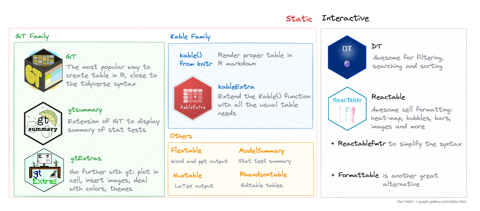
Figure: 4 big families used for table

GT

gt Standard

# library("gt")

# Create a simple data frame
data1 = data.frame(
  Country = c("USA", "China", "India", "Brazil"),
  Capitals = c("Washington D.C.", "Beijing", "New Delhi", "Brasília"),
  Population = c(331, 1441, 1393, 212),
  GDP = c(21.43, 14.34, 2.87, 1.49)
)

# Use the gt function
data1 %>% gt() %>%
  tab_header(title = md("What a **nice title**"),
             subtitle = md("Pretty *cool subtitle* too, `isn't it?`"))%>%
  tab_footnote(
    footnote = "Source: James & al., 2020",
    locations = cells_body(columns = Country, rows = 3)
  )

What a nice title
Pretty cool subtitle too, isn't it?
Country	Capitals	Population	GDP
USA	Washington D.C.	331	21.43
China	Beijing	1441	14.34
India1	New Delhi	1393	2.87
Brazil	Brasília	212	1.49
1 Source: James & al., 2020

gt Sub-header

The tab_spanner() function lets you group columns into categories.

data1 %>%
  gt() %>%
  tab_spanner(
    label = "Number",
    columns = c(GDP, Population)) %>%
  tab_spanner(
    label = "Label",
    columns = c(Country, Capitals)
  )

Label		Number
Country	Capitals	GDP	Population
USA	Washington D.C.	21.43	331
China	Beijing	14.34	1441
India	New Delhi	2.87	1393
Brazil	Brasília	1.49	212

gt Footer with mutliple references

data2 = data.frame(
  Planet = c("Earth", "Mars", "Jupiter", "Venus"),
  Moons = c(1, 2, 79, 0),
  Distance_from_Sun = c(149.6, 227.9, 778.3, 108.2),
  Diameter = c(12742, 6779, 139822, 12104)
)

data2 %>%
  gt() %>%
    tab_footnote(footnote = md("Measured in **millions** of Km"),
                 locations = cells_column_labels(columns = Distance_from_Sun)) %>%
    tab_footnote(footnote = md("Measured in **Km**"),
                 locations = cells_column_labels(columns = Diameter))

Planet	Moons	Distance_from_Sun1	Diameter2
Earth	1	149.6	12742
Mars	2	227.9	6779
Jupiter	79	778.3	139822
Venus	0	108.2	12104
1 Measured in millions of Km
2 Measured in Km

## Change the type of element that indicates the reference
data2 %>%
  gt() %>%
    tab_footnote(footnote = md("Measured in **millions** of Km"),
                 locations = cells_column_labels(columns = Distance_from_Sun)) %>%
    tab_footnote(footnote = md("Measured in **Km**"),
                 locations = cells_column_labels(columns = Diameter)) %>%
    tab_footnote(footnote = md("The original data are from *Some Organization*")) %>%
    opt_footnote_marks(marks = "LETTERS")

Planet	Moons	Distance_from_SunA	DiameterB
Earth	1	149.6	12742
Mars	2	227.9	6779
Jupiter	79	778.3	139822
Venus	0	108.2	12104
The original data are from Some Organization
A Measured in millions of Km
B Measured in Km

gt Customize titles

data3 = data.frame(
  Country = c("USA", "China", "India"),
  Capitals = c("Washington D.C.", "Beijing", "New Delhi"),
  Population = c(331, 1441, 1393),
  GDP = c(21.43, 14.34, 2.87)
)

# create and display the gt table 
data3 %>%
  gt() %>%
    tab_header(title = html("<span style='color:red;'>A <strong>red</strong> title</span>"),
               subtitle = md("This text will be *below the title* and is written in `markdown`"))

A red title
This text will be below the title and is written in markdown
Country	Capitals	Population	GDP
USA	Washington D.C.	331	21.43
China	Beijing	1441	14.34
India	New Delhi	1393	2.87

Reference

• Creating beautiful tables in R with {gt}
• citation("gt")

GTSUMMARY

gtSummary is a companion package to gt, specifically designed to enhance gt’s capabilities in summarizing statistical findings. It bridges the gap between data analysis and table creation, allowing users to seamlessly generate summary tables directly from their analytical outputs.

The gtsummary uses the tbl_summary() to generate the summary table and works well with the %>% symbol.

It automatically detects data type and use it to decides what type of statistics to compute. By default, it’s: - median, 1st and 3rd quartile for numeric columns - number of observations and proportion for categorical columns

gtsummary Continious Analysis

# create the general table
Orthodont %>% select(-Subject) %>% tbl_summary() 

Characteristic	N = 1081
distance	23.75 (22.00, 26.00)
age
8	27 (25%)
10	27 (25%)
12	27 (25%)
14	27 (25%)
Sex
Male	64 (59%)
Female	44 (41%)
Group
Subgroup A	53 (49%)
Subgroup B	55 (51%)
1 Median (Q1, Q3); n (%)

Orthodont %>% dplyr::select(-Subject) %>% 
  tbl_summary(by = Sex,  
              type = where(is.numeric) ~ "continuous2",
              statistic = all_continuous() ~ c("{mean} ({sd})", "{median} ({p25}, {p75})", "{min}, {max}"),
              label = list(distance = "Distance", age = "Age in years", missing = "no")) %>% 
  modify_header(label ~ "Variable") %>%
  modify_spanning_header(c("stat_1", "stat_2") ~ "Gender") %>%
  bold_labels() %>%
  # add_n() %>%
  add_overall() %>%
  add_p()

Variable	Overall N = 1081	Gender		p-value2
		Male N = 641	Female N = 441
Distance				<0.001
Mean (SD)	24.02 (2.93)	24.97 (2.90)	22.65 (2.40)
Median (Q1, Q3)	23.75 (22.00, 26.00)	24.75 (23.00, 26.50)	22.75 (21.00, 24.25)
Min, Max	16.50, 31.50	17.00, 31.50	16.50, 28.00
Age in years				>0.9
Mean (SD)	11.00 (2.25)	11.00 (2.25)	11.00 (2.26)
Median (Q1, Q3)	11.00 (9.00, 13.00)	11.00 (9.00, 13.00)	11.00 (9.00, 13.00)
Min, Max	8.00, 14.00	8.00, 14.00	8.00, 14.00
Group				0.5
Subgroup A	53 (49%)	33 (52%)	20 (45%)
Subgroup B	55 (51%)	31 (48%)	24 (55%)
1 n (%)
2 Wilcoxon rank sum test; Pearson’s Chi-squared test

gtsummary Categorical Analysis

Orthodont %>% dplyr::select(names(Orthodont_factor), -Subject) %>% 
  tbl_summary(by=Group,
              type = all_continuous() ~ "continuous2", 
              label = list(Sex = "Gender", missing = "no")) %>%
  modify_header(label ~ "Variable") %>%
  modify_spanning_header(c("stat_1", "stat_2") ~ "Subgroup") %>%
  bold_labels() %>%
  add_overall() 

Variable	Overall N = 1081	Subgroup
		Subgroup A N = 531	Subgroup B N = 551
Gender
Male	64 (59%)	33 (62%)	31 (56%)
Female	44 (41%)	20 (38%)	24 (44%)
1 n (%)

gtsummary Add a column based on a custom function

# create dataset
data("iris")
df = as.data.frame(iris)

my_anova = function(data, variable, by, ...) {
  result = aov(as.formula(paste(variable, "~", by)), data = data)
  summary(result)[[1]]$'Pr(>F)'[1] # Extracting the p-value for the group effect
}

# create the table
df %>%
  tbl_summary(by=Species) %>%
  add_overall() %>%
  add_p() %>%
  add_stat(fns = everything() ~ my_anova) %>%
  modify_header(
    list(
      add_stat_1 ~ "**p-value**",
      all_stat_cols() ~ "**{level}**"
    )
  ) %>%
  modify_footnote(
    add_stat_1 ~ "ANOVA")

Characteristic	Overall1	setosa1	versicolor1	virginica1	p-value2	p-value3
Sepal.Length	5.80 (5.10, 6.40)	5.00 (4.80, 5.20)	5.90 (5.60, 6.30)	6.50 (6.20, 6.90)	<0.001	0.000
Sepal.Width	3.00 (2.80, 3.30)	3.40 (3.20, 3.70)	2.80 (2.50, 3.00)	3.00 (2.80, 3.20)	<0.001	0.000
Petal.Length	4.35 (1.60, 5.10)	1.50 (1.40, 1.60)	4.35 (4.00, 4.60)	5.55 (5.10, 5.90)	<0.001	0.000
Petal.Width	1.30 (0.30, 1.80)	0.20 (0.20, 0.30)	1.30 (1.20, 1.50)	2.00 (1.80, 2.30)	<0.001	0.000
1 Median (Q1, Q3)
2 Kruskal-Wallis rank sum test
3 ANOVA

gtsummary Regression Result

data("Titanic")
df = as.data.frame(Titanic)# create the model

model <- glm(Survived ~ Age + Class + Sex + Freq,
             family=binomial, data=df)

# generate table 
model %>%
  tbl_regression(intercept=TRUE, conf.level=0.9) %>%
  add_glance_source_note() %>%
  add_global_p() %>%
  add_q() 

Characteristic	log(OR)1	90% CI1	p-value	q-value2
(Intercept)	0.10	-1.4, 1.6	>0.9	>0.9
Age			0.5	>0.9
Child	—	—
Adult	0.62	-0.78, 2.1
Class			>0.9	>0.9
1st	—	—
2nd	-0.03	-1.7, 1.7
3rd	0.25	-1.5, 2.0
Crew	0.27	-1.5, 2.0
Sex			0.6	>0.9
Male	—	—
Female	-0.37	-1.7, 0.89
Freq	-0.01	-0.02, 0.00	0.2	0.9
Null deviance = 44.4; Null df = 31; Log-likelihood = -21.3; AIC = 56.5; BIC = 66.8; Deviance = 42.5; Residual df = 25; No. Obs. = 32
1 OR = Odds Ratio, CI = Confidence Interval
2 False discovery rate correction for multiple testing

gtsummary Compare the Models

One easy way to show the results of 2 different models into a single table is to: - create a first table with the first model (logistic regression) - create a second table with the second model (Cox proportional hazards regression) - merge these tables with tbl_merge() - add a spanner for each model with the tab_spanner argument

# library("survival") 
data(trial)

model_reglog = glm(response ~ trt + grade, data=trial, family = binomial) %>% 
  tbl_regression()

model_cox = coxph(Surv(ttdeath, death) ~ trt + grade, data=trial) %>% 
  tbl_regression()

tbl_merge(
  list(model_reglog, model_cox),
  tab_spanner = c("**Tumor Response**", "**Time to Death**")
)

Characteristic	Tumor Response			Time to Death
	log(OR)1	95% CI1	p-value	log(HR)1	95% CI1	p-value
Chemotherapy Treatment
Drug A	—	—		—	—
Drug B	0.19	-0.41, 0.81	0.5	0.22	-0.15, 0.59	0.2
Grade
I	—	—		—	—
II	-0.06	-0.82, 0.68	0.9	0.25	-0.22, 0.72	0.3
III	0.08	-0.66, 0.82	0.8	0.52	0.07, 0.98	0.024
1 OR = Odds Ratio, CI = Confidence Interval, HR = Hazard Ratio

Reference

• Index
• CHEAT SHEET
• citation("gtsummary")
• browseVignettes("gtsummary")

GTEXTRAS

gtExtras augments and expands the functionalities of the gt package. It allows to create even more sophisticated and visually appealing tables.

gtExtras Data format

# load the dataset
data(iris)


# create aggregated dataset
agg_iris = iris %>%
  group_by(Species) %>%
  summarize(
    Sepal.L = list(Sepal.Length),
    Sepal.W = list(Sepal.Width),
    Petal.L = list(Petal.Length),
    Petal.W = list(Petal.Width)
    )

# display the table with default output with gt package
agg_iris %>%
  gt()

Species	Sepal.L	Sepal.W	Petal.L	Petal.W
setosa	5.1, 4.9, 4.7, 4.6, 5.0, 5.4, 4.6, 5.0, 4.4, 4.9, 5.4, 4.8, 4.8, 4.3, 5.8, 5.7, 5.4, 5.1, 5.7, 5.1, 5.4, 5.1, 4.6, 5.1, 4.8, 5.0, 5.0, 5.2, 5.2, 4.7, 4.8, 5.4, 5.2, 5.5, 4.9, 5.0, 5.5, 4.9, 4.4, 5.1, 5.0, 4.5, 4.4, 5.0, 5.1, 4.8, 5.1, 4.6, 5.3, 5.0	3.5, 3.0, 3.2, 3.1, 3.6, 3.9, 3.4, 3.4, 2.9, 3.1, 3.7, 3.4, 3.0, 3.0, 4.0, 4.4, 3.9, 3.5, 3.8, 3.8, 3.4, 3.7, 3.6, 3.3, 3.4, 3.0, 3.4, 3.5, 3.4, 3.2, 3.1, 3.4, 4.1, 4.2, 3.1, 3.2, 3.5, 3.6, 3.0, 3.4, 3.5, 2.3, 3.2, 3.5, 3.8, 3.0, 3.8, 3.2, 3.7, 3.3	1.4, 1.4, 1.3, 1.5, 1.4, 1.7, 1.4, 1.5, 1.4, 1.5, 1.5, 1.6, 1.4, 1.1, 1.2, 1.5, 1.3, 1.4, 1.7, 1.5, 1.7, 1.5, 1.0, 1.7, 1.9, 1.6, 1.6, 1.5, 1.4, 1.6, 1.6, 1.5, 1.5, 1.4, 1.5, 1.2, 1.3, 1.4, 1.3, 1.5, 1.3, 1.3, 1.3, 1.6, 1.9, 1.4, 1.6, 1.4, 1.5, 1.4	0.2, 0.2, 0.2, 0.2, 0.2, 0.4, 0.3, 0.2, 0.2, 0.1, 0.2, 0.2, 0.1, 0.1, 0.2, 0.4, 0.4, 0.3, 0.3, 0.3, 0.2, 0.4, 0.2, 0.5, 0.2, 0.2, 0.4, 0.2, 0.2, 0.2, 0.2, 0.4, 0.1, 0.2, 0.2, 0.2, 0.2, 0.1, 0.2, 0.2, 0.3, 0.3, 0.2, 0.6, 0.4, 0.3, 0.2, 0.2, 0.2, 0.2
versicolor	7.0, 6.4, 6.9, 5.5, 6.5, 5.7, 6.3, 4.9, 6.6, 5.2, 5.0, 5.9, 6.0, 6.1, 5.6, 6.7, 5.6, 5.8, 6.2, 5.6, 5.9, 6.1, 6.3, 6.1, 6.4, 6.6, 6.8, 6.7, 6.0, 5.7, 5.5, 5.5, 5.8, 6.0, 5.4, 6.0, 6.7, 6.3, 5.6, 5.5, 5.5, 6.1, 5.8, 5.0, 5.6, 5.7, 5.7, 6.2, 5.1, 5.7	3.2, 3.2, 3.1, 2.3, 2.8, 2.8, 3.3, 2.4, 2.9, 2.7, 2.0, 3.0, 2.2, 2.9, 2.9, 3.1, 3.0, 2.7, 2.2, 2.5, 3.2, 2.8, 2.5, 2.8, 2.9, 3.0, 2.8, 3.0, 2.9, 2.6, 2.4, 2.4, 2.7, 2.7, 3.0, 3.4, 3.1, 2.3, 3.0, 2.5, 2.6, 3.0, 2.6, 2.3, 2.7, 3.0, 2.9, 2.9, 2.5, 2.8	4.7, 4.5, 4.9, 4.0, 4.6, 4.5, 4.7, 3.3, 4.6, 3.9, 3.5, 4.2, 4.0, 4.7, 3.6, 4.4, 4.5, 4.1, 4.5, 3.9, 4.8, 4.0, 4.9, 4.7, 4.3, 4.4, 4.8, 5.0, 4.5, 3.5, 3.8, 3.7, 3.9, 5.1, 4.5, 4.5, 4.7, 4.4, 4.1, 4.0, 4.4, 4.6, 4.0, 3.3, 4.2, 4.2, 4.2, 4.3, 3.0, 4.1	1.4, 1.5, 1.5, 1.3, 1.5, 1.3, 1.6, 1.0, 1.3, 1.4, 1.0, 1.5, 1.0, 1.4, 1.3, 1.4, 1.5, 1.0, 1.5, 1.1, 1.8, 1.3, 1.5, 1.2, 1.3, 1.4, 1.4, 1.7, 1.5, 1.0, 1.1, 1.0, 1.2, 1.6, 1.5, 1.6, 1.5, 1.3, 1.3, 1.3, 1.2, 1.4, 1.2, 1.0, 1.3, 1.2, 1.3, 1.3, 1.1, 1.3
virginica	6.3, 5.8, 7.1, 6.3, 6.5, 7.6, 4.9, 7.3, 6.7, 7.2, 6.5, 6.4, 6.8, 5.7, 5.8, 6.4, 6.5, 7.7, 7.7, 6.0, 6.9, 5.6, 7.7, 6.3, 6.7, 7.2, 6.2, 6.1, 6.4, 7.2, 7.4, 7.9, 6.4, 6.3, 6.1, 7.7, 6.3, 6.4, 6.0, 6.9, 6.7, 6.9, 5.8, 6.8, 6.7, 6.7, 6.3, 6.5, 6.2, 5.9	3.3, 2.7, 3.0, 2.9, 3.0, 3.0, 2.5, 2.9, 2.5, 3.6, 3.2, 2.7, 3.0, 2.5, 2.8, 3.2, 3.0, 3.8, 2.6, 2.2, 3.2, 2.8, 2.8, 2.7, 3.3, 3.2, 2.8, 3.0, 2.8, 3.0, 2.8, 3.8, 2.8, 2.8, 2.6, 3.0, 3.4, 3.1, 3.0, 3.1, 3.1, 3.1, 2.7, 3.2, 3.3, 3.0, 2.5, 3.0, 3.4, 3.0	6.0, 5.1, 5.9, 5.6, 5.8, 6.6, 4.5, 6.3, 5.8, 6.1, 5.1, 5.3, 5.5, 5.0, 5.1, 5.3, 5.5, 6.7, 6.9, 5.0, 5.7, 4.9, 6.7, 4.9, 5.7, 6.0, 4.8, 4.9, 5.6, 5.8, 6.1, 6.4, 5.6, 5.1, 5.6, 6.1, 5.6, 5.5, 4.8, 5.4, 5.6, 5.1, 5.1, 5.9, 5.7, 5.2, 5.0, 5.2, 5.4, 5.1	2.5, 1.9, 2.1, 1.8, 2.2, 2.1, 1.7, 1.8, 1.8, 2.5, 2.0, 1.9, 2.1, 2.0, 2.4, 2.3, 1.8, 2.2, 2.3, 1.5, 2.3, 2.0, 2.0, 1.8, 2.1, 1.8, 1.8, 1.8, 2.1, 1.6, 1.9, 2.0, 2.2, 1.5, 1.4, 2.3, 2.4, 1.8, 1.8, 2.1, 2.4, 2.3, 1.9, 2.3, 2.5, 2.3, 1.9, 2.0, 2.3, 1.8

gtExtras Change Theme

## Excel theme
head(mtcars) %>%
  gt() %>%
  gt_theme_excel()

mpg	cyl	disp	hp	drat	wt	qsec	vs	am	gear	carb
21.0	6	160	110	3.90	2.620	16.46	0	1	4	4
21.0	6	160	110	3.90	2.875	17.02	0	1	4	4
22.8	4	108	93	3.85	2.320	18.61	1	1	4	1
21.4	6	258	110	3.08	3.215	19.44	1	0	3	1
18.7	8	360	175	3.15	3.440	17.02	0	0	3	2
18.1	6	225	105	2.76	3.460	20.22	1	0	3	1

## FiveThirtyEight theme
head(mtcars) %>%
  gt() %>%
  gt_theme_538()

mpg	cyl	disp	hp	drat	wt	qsec	vs	am	gear	carb
21.0	6	160	110	3.90	2.620	16.46	0	1	4	4
21.0	6	160	110	3.90	2.875	17.02	0	1	4	4
22.8	4	108	93	3.85	2.320	18.61	1	1	4	1
21.4	6	258	110	3.08	3.215	19.44	1	0	3	1
18.7	8	360	175	3.15	3.440	17.02	0	0	3	2
18.1	6	225	105	2.76	3.460	20.22	1	0	3	1

## ESPN theme
head(mtcars) %>%
  gt() %>%
  gt_theme_espn()

mpg	cyl	disp	hp	drat	wt	qsec	vs	am	gear	carb
21.0	6	160	110	3.90	2.620	16.46	0	1	4	4
21.0	6	160	110	3.90	2.875	17.02	0	1	4	4
22.8	4	108	93	3.85	2.320	18.61	1	1	4	1
21.4	6	258	110	3.08	3.215	19.44	1	0	3	1
18.7	8	360	175	3.15	3.440	17.02	0	0	3	2
18.1	6	225	105	2.76	3.460	20.22	1	0	3	1

## NY Times theme
head(mtcars) %>%
  gt() %>%
  gt_theme_nytimes()

mpg	cyl	disp	hp	drat	wt	qsec	vs	am	gear	carb
21.0	6	160	110	3.90	2.620	16.46	0	1	4	4
21.0	6	160	110	3.90	2.875	17.02	0	1	4	4
22.8	4	108	93	3.85	2.320	18.61	1	1	4	1
21.4	6	258	110	3.08	3.215	19.44	1	0	3	1
18.7	8	360	175	3.15	3.440	17.02	0	0	3	2
18.1	6	225	105	2.76	3.460	20.22	1	0	3	1

## Dot matrix theme
head(mtcars) %>%
  gt() %>%
  gt_theme_dot_matrix()

mpg	cyl	disp	hp	drat	wt	qsec	vs	am	gear	carb
21.0	6	160	110	3.90	2.620	16.46	0	1	4	4
21.0	6	160	110	3.90	2.875	17.02	0	1	4	4
22.8	4	108	93	3.85	2.320	18.61	1	1	4	1
21.4	6	258	110	3.08	3.215	19.44	1	0	3	1
18.7	8	360	175	3.15	3.440	17.02	0	0	3	2
18.1	6	225	105	2.76	3.460	20.22	1	0	3	1

## Dark theme
head(mtcars) %>%
  gt() %>%
  gt_theme_dark()

mpg	cyl	disp	hp	drat	wt	qsec	vs	am	gear	carb
21.0	6	160	110	3.90	2.620	16.46	0	1	4	4
21.0	6	160	110	3.90	2.875	17.02	0	1	4	4
22.8	4	108	93	3.85	2.320	18.61	1	1	4	1
21.4	6	258	110	3.08	3.215	19.44	1	0	3	1
18.7	8	360	175	3.15	3.440	17.02	0	0	3	2
18.1	6	225	105	2.76	3.460	20.22	1	0	3	1

## PFF theme
head(mtcars) %>%
  gt() %>%
  gt_theme_pff()

mpg	cyl	disp	hp	drat	wt	qsec	vs	am	gear	carb
21.0	6	160	110	3.90	2.620	16.46	0	1	4	4
21.0	6	160	110	3.90	2.875	17.02	0	1	4	4
22.8	4	108	93	3.85	2.320	18.61	1	1	4	1
21.4	6	258	110	3.08	3.215	19.44	1	0	3	1
18.7	8	360	175	3.15	3.440	17.02	0	0	3	2
18.1	6	225	105	2.76	3.460	20.22	1	0	3	1

## Guardian theme
head(mtcars) %>%
  gt() %>%
  gt_theme_guardian()

mpg	cyl	disp	hp	drat	wt	qsec	vs	am	gear	carb
21.0	6	160	110	3.90	2.620	16.46	0	1	4	4
21.0	6	160	110	3.90	2.875	17.02	0	1	4	4
22.8	4	108	93	3.85	2.320	18.61	1	1	4	1
21.4	6	258	110	3.08	3.215	19.44	1	0	3	1
18.7	8	360	175	3.15	3.440	17.02	0	0	3	2
18.1	6	225	105	2.76	3.460	20.22	1	0	3	1

gtExtras Chart within Table

• gt_plt_sparkline() creates a line chart in table cells.
• gt_plt_dist() creates a distribution chart chart in table cells

agg_iris %>%
  gt() %>%
  gt_plt_sparkline(Sepal.L) %>%
  gt_plt_dist(Sepal.W, type = "density") %>%
  gt_plt_dist(Petal.L, type = "boxplot") %>%
  gt_plt_dist(Petal.W, type = "histogram")

Species	Sepal.L	Sepal.W	Petal.L	Petal.W
setosa
versicolor
virginica

gtExtras Summary chart

iris %>%
  gt_plt_summary() 

.
150 rows x 5 cols
	Column	Plot Overview	Missing	Mean	Median	SD
	Sepal.Length		0.0%	5.8	5.8	0.8
	Sepal.Width		0.0%	3.1	3.0	0.4
	Petal.Length		0.0%	3.8	4.3	1.8
	Petal.Width		0.0%	1.2	1.3	0.8
	Species setosa, versicolor and virginica		0.0%	—	—	—

Referecne

• citation("gtExtras")

KABLEEXTRA and KABLE

kableExtra Standard

When used on a HTML table, kable_styling() will automatically apply twitter bootstrap theme to the table. Now it should looks the same as the original pandoc output (the one when you don’t specify format in kable()) but this time, you are controlling it.

• By default, full_width is set to be TRUE for HTML tables
• Position: align the table to center, left or right side of the page

dt <- mtcars[1:5, 1:6]

### Bootstrap theme
library("naniar")
airquality %>% 
  miss_var_summary() %>%
  kable(caption = "Missing data among variables", format = "html") %>%
  add_footnote(c("Footnote 1: XXX")) %>%
  kable_styling(bootstrap_options = "striped", 
                full_width = F, 
                position = "center",
                fixed_thead = T) 

Missing data among variables

variable	n_miss	pct_miss
Ozone	37	24.2
Solar.R	7	4.58
Wind	0	0
Temp	0	0
Month	0	0
Day	0	0
a Footnote 1: XXX

airquality %>% 
  miss_var_summary() %>%
  kable(caption = "Missing data among variables", format = "html") %>%
  add_footnote(c("Footnote 1: XXX")) %>%
  kable_styling(bootstrap_options = "striped", full_width = F, position = "float_right") 

Missing data among variables

variable	n_miss	pct_miss
Ozone	37	24.2
Solar.R	7	4.58
Wind	0	0
Temp	0	0
Month	0	0
Day	0	0
a Footnote 1: XXX

Becides these three common options, you can also wrap text around the table using the float-left or float-right options.

kableExtra Table Footnote

kbl(dt, align = "c") %>%
  kable_classic(full_width = F) %>%
  footnote(general = "Here is a general comments of the table. ",
           number = c("Footnote 1; ", "Footnote 2; "),
           alphabet = c("Footnote A; ", "Footnote B; "),
           symbol = c("Footnote Symbol 1; ", "Footnote Symbol 2")
           )

	mpg	cyl	disp	hp	drat	wt
Mazda RX4	21.0	6	160	110	3.90	2.620
Mazda RX4 Wag	21.0	6	160	110	3.90	2.875
Datsun 710	22.8	4	108	93	3.85	2.320
Hornet 4 Drive	21.4	6	258	110	3.08	3.215
Hornet Sportabout	18.7	8	360	175	3.15	3.440
Note:
Here is a general comments of the table.
1 Footnote 1;
2 Footnote 2;
a Footnote A;
b Footnote B;
* Footnote Symbol 1;
† Footnote Symbol 2

kableExtra Scroll Box

kbl(cbind(mtcars, mtcars)) %>%
  kable_paper() %>%
  scroll_box(width = "500px", height = "200px")

	mpg	cyl	disp	hp	drat	wt	qsec	vs	am	gear	carb	mpg	cyl	disp	hp	drat	wt	qsec	vs	am	gear	carb
Mazda RX4	21.0	6	160.0	110	3.90	2.620	16.46	0	1	4	4	21.0	6	160.0	110	3.90	2.620	16.46	0	1	4	4
Mazda RX4 Wag	21.0	6	160.0	110	3.90	2.875	17.02	0	1	4	4	21.0	6	160.0	110	3.90	2.875	17.02	0	1	4	4
Datsun 710	22.8	4	108.0	93	3.85	2.320	18.61	1	1	4	1	22.8	4	108.0	93	3.85	2.320	18.61	1	1	4	1
Hornet 4 Drive	21.4	6	258.0	110	3.08	3.215	19.44	1	0	3	1	21.4	6	258.0	110	3.08	3.215	19.44	1	0	3	1
Hornet Sportabout	18.7	8	360.0	175	3.15	3.440	17.02	0	0	3	2	18.7	8	360.0	175	3.15	3.440	17.02	0	0	3	2
Valiant	18.1	6	225.0	105	2.76	3.460	20.22	1	0	3	1	18.1	6	225.0	105	2.76	3.460	20.22	1	0	3	1
Duster 360	14.3	8	360.0	245	3.21	3.570	15.84	0	0	3	4	14.3	8	360.0	245	3.21	3.570	15.84	0	0	3	4
Merc 240D	24.4	4	146.7	62	3.69	3.190	20.00	1	0	4	2	24.4	4	146.7	62	3.69	3.190	20.00	1	0	4	2
Merc 230	22.8	4	140.8	95	3.92	3.150	22.90	1	0	4	2	22.8	4	140.8	95	3.92	3.150	22.90	1	0	4	2
Merc 280	19.2	6	167.6	123	3.92	3.440	18.30	1	0	4	4	19.2	6	167.6	123	3.92	3.440	18.30	1	0	4	4
Merc 280C	17.8	6	167.6	123	3.92	3.440	18.90	1	0	4	4	17.8	6	167.6	123	3.92	3.440	18.90	1	0	4	4
Merc 450SE	16.4	8	275.8	180	3.07	4.070	17.40	0	0	3	3	16.4	8	275.8	180	3.07	4.070	17.40	0	0	3	3
Merc 450SL	17.3	8	275.8	180	3.07	3.730	17.60	0	0	3	3	17.3	8	275.8	180	3.07	3.730	17.60	0	0	3	3
Merc 450SLC	15.2	8	275.8	180	3.07	3.780	18.00	0	0	3	3	15.2	8	275.8	180	3.07	3.780	18.00	0	0	3	3
Cadillac Fleetwood	10.4	8	472.0	205	2.93	5.250	17.98	0	0	3	4	10.4	8	472.0	205	2.93	5.250	17.98	0	0	3	4
Lincoln Continental	10.4	8	460.0	215	3.00	5.424	17.82	0	0	3	4	10.4	8	460.0	215	3.00	5.424	17.82	0	0	3	4
Chrysler Imperial	14.7	8	440.0	230	3.23	5.345	17.42	0	0	3	4	14.7	8	440.0	230	3.23	5.345	17.42	0	0	3	4
Fiat 128	32.4	4	78.7	66	4.08	2.200	19.47	1	1	4	1	32.4	4	78.7	66	4.08	2.200	19.47	1	1	4	1
Honda Civic	30.4	4	75.7	52	4.93	1.615	18.52	1	1	4	2	30.4	4	75.7	52	4.93	1.615	18.52	1	1	4	2
Toyota Corolla	33.9	4	71.1	65	4.22	1.835	19.90	1	1	4	1	33.9	4	71.1	65	4.22	1.835	19.90	1	1	4	1
Toyota Corona	21.5	4	120.1	97	3.70	2.465	20.01	1	0	3	1	21.5	4	120.1	97	3.70	2.465	20.01	1	0	3	1
Dodge Challenger	15.5	8	318.0	150	2.76	3.520	16.87	0	0	3	2	15.5	8	318.0	150	2.76	3.520	16.87	0	0	3	2
AMC Javelin	15.2	8	304.0	150	3.15	3.435	17.30	0	0	3	2	15.2	8	304.0	150	3.15	3.435	17.30	0	0	3	2
Camaro Z28	13.3	8	350.0	245	3.73	3.840	15.41	0	0	3	4	13.3	8	350.0	245	3.73	3.840	15.41	0	0	3	4
Pontiac Firebird	19.2	8	400.0	175	3.08	3.845	17.05	0	0	3	2	19.2	8	400.0	175	3.08	3.845	17.05	0	0	3	2
Fiat X1-9	27.3	4	79.0	66	4.08	1.935	18.90	1	1	4	1	27.3	4	79.0	66	4.08	1.935	18.90	1	1	4	1
Porsche 914-2	26.0	4	120.3	91	4.43	2.140	16.70	0	1	5	2	26.0	4	120.3	91	4.43	2.140	16.70	0	1	5	2
Lotus Europa	30.4	4	95.1	113	3.77	1.513	16.90	1	1	5	2	30.4	4	95.1	113	3.77	1.513	16.90	1	1	5	2
Ford Pantera L	15.8	8	351.0	264	4.22	3.170	14.50	0	1	5	4	15.8	8	351.0	264	4.22	3.170	14.50	0	1	5	4
Ferrari Dino	19.7	6	145.0	175	3.62	2.770	15.50	0	1	5	6	19.7	6	145.0	175	3.62	2.770	15.50	0	1	5	6
Maserati Bora	15.0	8	301.0	335	3.54	3.570	14.60	0	1	5	8	15.0	8	301.0	335	3.54	3.570	14.60	0	1	5	8
Volvo 142E	21.4	4	121.0	109	4.11	2.780	18.60	1	1	4	2	21.4	4	121.0	109	4.11	2.780	18.60	1	1	4	2

kbl(cbind(mtcars, mtcars)) %>%
  add_header_above(c("a" = 5, "b" = 18)) %>%
  kable_paper() %>%
  scroll_box(width = "100%", height = "200px")

a					b
	mpg	cyl	disp	hp	drat	wt	qsec	vs	am	gear	carb	mpg	cyl	disp	hp	drat	wt	qsec	vs	am	gear	carb
Mazda RX4	21.0	6	160.0	110	3.90	2.620	16.46	0	1	4	4	21.0	6	160.0	110	3.90	2.620	16.46	0	1	4	4
Mazda RX4 Wag	21.0	6	160.0	110	3.90	2.875	17.02	0	1	4	4	21.0	6	160.0	110	3.90	2.875	17.02	0	1	4	4
Datsun 710	22.8	4	108.0	93	3.85	2.320	18.61	1	1	4	1	22.8	4	108.0	93	3.85	2.320	18.61	1	1	4	1
Hornet 4 Drive	21.4	6	258.0	110	3.08	3.215	19.44	1	0	3	1	21.4	6	258.0	110	3.08	3.215	19.44	1	0	3	1
Hornet Sportabout	18.7	8	360.0	175	3.15	3.440	17.02	0	0	3	2	18.7	8	360.0	175	3.15	3.440	17.02	0	0	3	2
Valiant	18.1	6	225.0	105	2.76	3.460	20.22	1	0	3	1	18.1	6	225.0	105	2.76	3.460	20.22	1	0	3	1
Duster 360	14.3	8	360.0	245	3.21	3.570	15.84	0	0	3	4	14.3	8	360.0	245	3.21	3.570	15.84	0	0	3	4
Merc 240D	24.4	4	146.7	62	3.69	3.190	20.00	1	0	4	2	24.4	4	146.7	62	3.69	3.190	20.00	1	0	4	2
Merc 230	22.8	4	140.8	95	3.92	3.150	22.90	1	0	4	2	22.8	4	140.8	95	3.92	3.150	22.90	1	0	4	2
Merc 280	19.2	6	167.6	123	3.92	3.440	18.30	1	0	4	4	19.2	6	167.6	123	3.92	3.440	18.30	1	0	4	4
Merc 280C	17.8	6	167.6	123	3.92	3.440	18.90	1	0	4	4	17.8	6	167.6	123	3.92	3.440	18.90	1	0	4	4
Merc 450SE	16.4	8	275.8	180	3.07	4.070	17.40	0	0	3	3	16.4	8	275.8	180	3.07	4.070	17.40	0	0	3	3
Merc 450SL	17.3	8	275.8	180	3.07	3.730	17.60	0	0	3	3	17.3	8	275.8	180	3.07	3.730	17.60	0	0	3	3
Merc 450SLC	15.2	8	275.8	180	3.07	3.780	18.00	0	0	3	3	15.2	8	275.8	180	3.07	3.780	18.00	0	0	3	3
Cadillac Fleetwood	10.4	8	472.0	205	2.93	5.250	17.98	0	0	3	4	10.4	8	472.0	205	2.93	5.250	17.98	0	0	3	4
Lincoln Continental	10.4	8	460.0	215	3.00	5.424	17.82	0	0	3	4	10.4	8	460.0	215	3.00	5.424	17.82	0	0	3	4
Chrysler Imperial	14.7	8	440.0	230	3.23	5.345	17.42	0	0	3	4	14.7	8	440.0	230	3.23	5.345	17.42	0	0	3	4
Fiat 128	32.4	4	78.7	66	4.08	2.200	19.47	1	1	4	1	32.4	4	78.7	66	4.08	2.200	19.47	1	1	4	1
Honda Civic	30.4	4	75.7	52	4.93	1.615	18.52	1	1	4	2	30.4	4	75.7	52	4.93	1.615	18.52	1	1	4	2
Toyota Corolla	33.9	4	71.1	65	4.22	1.835	19.90	1	1	4	1	33.9	4	71.1	65	4.22	1.835	19.90	1	1	4	1
Toyota Corona	21.5	4	120.1	97	3.70	2.465	20.01	1	0	3	1	21.5	4	120.1	97	3.70	2.465	20.01	1	0	3	1
Dodge Challenger	15.5	8	318.0	150	2.76	3.520	16.87	0	0	3	2	15.5	8	318.0	150	2.76	3.520	16.87	0	0	3	2
AMC Javelin	15.2	8	304.0	150	3.15	3.435	17.30	0	0	3	2	15.2	8	304.0	150	3.15	3.435	17.30	0	0	3	2
Camaro Z28	13.3	8	350.0	245	3.73	3.840	15.41	0	0	3	4	13.3	8	350.0	245	3.73	3.840	15.41	0	0	3	4
Pontiac Firebird	19.2	8	400.0	175	3.08	3.845	17.05	0	0	3	2	19.2	8	400.0	175	3.08	3.845	17.05	0	0	3	2
Fiat X1-9	27.3	4	79.0	66	4.08	1.935	18.90	1	1	4	1	27.3	4	79.0	66	4.08	1.935	18.90	1	1	4	1
Porsche 914-2	26.0	4	120.3	91	4.43	2.140	16.70	0	1	5	2	26.0	4	120.3	91	4.43	2.140	16.70	0	1	5	2
Lotus Europa	30.4	4	95.1	113	3.77	1.513	16.90	1	1	5	2	30.4	4	95.1	113	3.77	1.513	16.90	1	1	5	2
Ford Pantera L	15.8	8	351.0	264	4.22	3.170	14.50	0	1	5	4	15.8	8	351.0	264	4.22	3.170	14.50	0	1	5	4
Ferrari Dino	19.7	6	145.0	175	3.62	2.770	15.50	0	1	5	6	19.7	6	145.0	175	3.62	2.770	15.50	0	1	5	6
Maserati Bora	15.0	8	301.0	335	3.54	3.570	14.60	0	1	5	8	15.0	8	301.0	335	3.54	3.570	14.60	0	1	5	8
Volvo 142E	21.4	4	121.0	109	4.11	2.780	18.60	1	1	4	2	21.4	4	121.0	109	4.11	2.780	18.60	1	1	4	2

kableExtra Change Thema

kableExtra also offers a few in-house alternative HTML table themes other than the default bootstrap theme. Right now there are 6 of them: kable_paper, kable_classic, kable_classic_2, kable_minimal, kable_material and kable_material_dark. These functions are alternatives to kable_styling, which means that you can specify any additional formatting options in kable_styling in these functions too. The only difference is that bootstrap_options (as discussed in the next section) is replaced with lightable_options at the same location with only two choices striped and hover available.

head(iris) %>%
  kbl() %>%
  kable_paper("hover", full_width = F)

Sepal.Length	Sepal.Width	Petal.Length	Petal.Width	Species
5.1	3.5	1.4	0.2	setosa
4.9	3.0	1.4	0.2	setosa
4.7	3.2	1.3	0.2	setosa
4.6	3.1	1.5	0.2	setosa
5.0	3.6	1.4	0.2	setosa
5.4	3.9	1.7	0.4	setosa

head(iris) %>%
  kbl(caption = "Recreating booktabs style table") %>%
  kable_classic(full_width = F, html_font = "Cambria")

Recreating booktabs style table

Sepal.Length	Sepal.Width	Petal.Length	Petal.Width	Species
5.1	3.5	1.4	0.2	setosa
4.9	3.0	1.4	0.2	setosa
4.7	3.2	1.3	0.2	setosa
4.6	3.1	1.5	0.2	setosa
5.0	3.6	1.4	0.2	setosa
5.4	3.9	1.7	0.4	setosa

head(iris) %>%
  kbl() %>%
  kable_classic_2(full_width = F)

Sepal.Length	Sepal.Width	Petal.Length	Petal.Width	Species
5.1	3.5	1.4	0.2	setosa
4.9	3.0	1.4	0.2	setosa
4.7	3.2	1.3	0.2	setosa
4.6	3.1	1.5	0.2	setosa
5.0	3.6	1.4	0.2	setosa
5.4	3.9	1.7	0.4	setosa

head(iris) %>%
  kbl() %>%
  kable_minimal()

Sepal.Length	Sepal.Width	Petal.Length	Petal.Width	Species
5.1	3.5	1.4	0.2	setosa
4.9	3.0	1.4	0.2	setosa
4.7	3.2	1.3	0.2	setosa
4.6	3.1	1.5	0.2	setosa
5.0	3.6	1.4	0.2	setosa
5.4	3.9	1.7	0.4	setosa

head(iris) %>%
  kbl() %>%
  kable_material(c("striped", "hover"))

Sepal.Length	Sepal.Width	Petal.Length	Petal.Width	Species
5.1	3.5	1.4	0.2	setosa
4.9	3.0	1.4	0.2	setosa
4.7	3.2	1.3	0.2	setosa
4.6	3.1	1.5	0.2	setosa
5.0	3.6	1.4	0.2	setosa
5.4	3.9	1.7	0.4	setosa

head(iris) %>%
  kbl() %>%
  kable_material_dark()

Sepal.Length	Sepal.Width	Petal.Length	Petal.Width	Species
5.1	3.5	1.4	0.2	setosa
4.9	3.0	1.4	0.2	setosa
4.7	3.2	1.3	0.2	setosa
4.6	3.1	1.5	0.2	setosa
5.0	3.6	1.4	0.2	setosa
5.4	3.9	1.7	0.4	setosa

kableExtra Bootstrap table classes

Predefined classes, including striped, bordered, hover, condensed and responsive

• The option condensed can also be handy in many cases when you don’t want your table to be too large. It has slightly shorter row height.
• Tables with option responsive looks the same with others on a large screen. However, on a small screen like phone, they are horizontally scrollable. Please resize your window to see the result.

kbl(head(iris)) %>%
  kable_styling(bootstrap_options = c("striped", "hover"))

Sepal.Length	Sepal.Width	Petal.Length	Petal.Width	Species
5.1	3.5	1.4	0.2	setosa
4.9	3.0	1.4	0.2	setosa
4.7	3.2	1.3	0.2	setosa
4.6	3.1	1.5	0.2	setosa
5.0	3.6	1.4	0.2	setosa
5.4	3.9	1.7	0.4	setosa

kbl(head(iris)) %>%
  kable_styling(bootstrap_options = c("bordered", "hover"))

Sepal.Length	Sepal.Width	Petal.Length	Petal.Width	Species
5.1	3.5	1.4	0.2	setosa
4.9	3.0	1.4	0.2	setosa
4.7	3.2	1.3	0.2	setosa
4.6	3.1	1.5	0.2	setosa
5.0	3.6	1.4	0.2	setosa
5.4	3.9	1.7	0.4	setosa

kbl(head(iris)) %>%
  kable_styling(bootstrap_options = c("striped","condensed", "hover"))

Sepal.Length	Sepal.Width	Petal.Length	Petal.Width	Species
5.1	3.5	1.4	0.2	setosa
4.9	3.0	1.4	0.2	setosa
4.7	3.2	1.3	0.2	setosa
4.6	3.1	1.5	0.2	setosa
5.0	3.6	1.4	0.2	setosa
5.4	3.9	1.7	0.4	setosa

kbl(head(iris))%>%
  kable_styling(bootstrap_options = c("striped", "hover", "condensed", "responsive"))

Sepal.Length	Sepal.Width	Petal.Length	Petal.Width	Species
5.1	3.5	1.4	0.2	setosa
4.9	3.0	1.4	0.2	setosa
4.7	3.2	1.3	0.2	setosa
4.6	3.1	1.5	0.2	setosa
5.0	3.6	1.4	0.2	setosa
5.4	3.9	1.7	0.4	setosa

kableExtra Column Specification

mtcars[1:8, 1:8] %>%
  kbl() %>%
  kable_paper(full_width = F) %>%
  column_spec(2, color = spec_color(mtcars$mpg[1:8]),
              link = "https://haozhu233.github.io/kableExtra/") %>%
  column_spec(6, color = "white",
              background = spec_color(mtcars$drat[1:8], end = 0.7),
              popover = paste("am:", mtcars$am[1:8]))

	mpg	cyl	disp	hp	drat	wt	qsec	vs
Mazda RX4	21.0	6	160.0	110	3.90	2.620	16.46	0
Mazda RX4 Wag	21.0	6	160.0	110	3.90	2.875	17.02	0
Datsun 710	22.8	4	108.0	93	3.85	2.320	18.61	1
Hornet 4 Drive	21.4	6	258.0	110	3.08	3.215	19.44	1
Hornet Sportabout	18.7	8	360.0	175	3.15	3.440	17.02	0
Valiant	18.1	6	225.0	105	2.76	3.460	20.22	1
Duster 360	14.3	8	360.0	245	3.21	3.570	15.84	0
Merc 240D	24.4	4	146.7	62	3.69	3.190	20.00	1

kableExtra Insert Images into Columns

kableExtra also provides a few inline plotting tools. Right now, there are spec_hist, spec_boxplot, and spec_plot. One key feature is that by default, the limits of every subplots are fixed so you can compare across rows. Note that in html, you can also use package sparkline to create some jquery based interactive sparklines. Check out the end of this guide for details.

mpg_list <- split(mtcars$mpg, mtcars$cyl)
disp_list <- split(mtcars$disp, mtcars$cyl)
inline_plot <- data.frame(cyl = c(4, 6, 8), mpg_box = "", mpg_hist = "",
                          mpg_line1 = "", mpg_line2 = "",
                          mpg_points1 = "", mpg_points2 = "", mpg_poly = "")
inline_plot %>%
  kbl(booktabs = TRUE) %>%
  kable_paper(full_width = FALSE) %>%
  column_spec(2, image = spec_boxplot(mpg_list)) %>%
  column_spec(3, image = spec_hist(mpg_list)) %>%
  column_spec(4, image = spec_plot(mpg_list, same_lim = TRUE)) %>%
  column_spec(5, image = spec_plot(mpg_list, same_lim = FALSE)) %>%
  column_spec(6, image = spec_plot(mpg_list, type = "p")) %>%
  column_spec(7, image = spec_plot(mpg_list, disp_list, type = "p")) %>%
  column_spec(8, image = spec_plot(mpg_list, polymin = 5))

cyl	mpg_box	mpg_hist	mpg_line1	mpg_line2	mpg_points1	mpg_points2	mpg_poly
4
6
8

There is also a spec_pointrange function specifically designed for forest plots in regression tables. Of course, feel free to use it for other purposes.

coef_table <- data.frame(
  Variables = c("var 1", "var 2", "var 3"),
  Coefficients = c(1.6, 0.2, -2.0),
  Conf.Lower = c(1.3, -0.4, -2.5),
  Conf.Higher = c(1.9, 0.6, -1.4)
) 

data.frame(
  Variable = coef_table$Variables,
  Visualization = ""
) %>%
  kbl(booktabs = T) %>%
  kable_classic(full_width = FALSE) %>%
  column_spec(2, image = spec_pointrange(
    x = coef_table$Coefficients, 
    xmin = coef_table$Conf.Lower, 
    xmax = coef_table$Conf.Higher, 
    vline = 0)
    )

Variable	Visualization
var 1
var 2
var 3

kableExtra Row Specification

kbl(head(iris)) %>%
  kable_paper("striped", full_width = F) %>%
  column_spec(3:4, bold = T) %>%
  row_spec(3:5, bold = T, color = "white", background = "#D7261E")

Sepal.Length	Sepal.Width	Petal.Length	Petal.Width	Species
5.1	3.5	1.4	0.2	setosa
4.9	3.0	1.4	0.2	setosa
4.7	3.2	1.3	0.2	setosa
4.6	3.1	1.5	0.2	setosa
5.0	3.6	1.4	0.2	setosa
5.4	3.9	1.7	0.4	setosa

kableExtra Grouped Columns/Rows

Tables with multi-row headers can be very useful to demonstrate grouped data. To do that, you can pipe your kable object into add_header_above(). The header variable is supposed to be a named character with the names as new column names and values as column span. For your convenience, if column span equals to 1, you can ignore the =1 part so the function below can be written as `add_header_above(c(” “,”Group 1” = 2, “Group 2” = 2, “Group 3” = 2)).

kbl(dt) %>%
  kable_classic() %>%
  add_header_above(c(" " = 1, "Group 1" = 2, "Group 2" = 2, "Group 3" = 2))

	Group 1		Group 2		Group 3
	mpg	cyl	disp	hp	drat	wt
Mazda RX4	21.0	6	160	110	3.90	2.620
Mazda RX4 Wag	21.0	6	160	110	3.90	2.875
Datsun 710	22.8	4	108	93	3.85	2.320
Hornet 4 Drive	21.4	6	258	110	3.08	3.215
Hornet Sportabout	18.7	8	360	175	3.15	3.440

kbl(dt) %>%
  kable_paper() %>%
  add_header_above(c(" ", "Group 1" = 2, "Group 2" = 2, "Group 3" = 2)) %>%
  add_header_above(c(" ", "Group 4" = 4, "Group 5" = 2)) %>%
  add_header_above(c(" ", "Group 6" = 6))

	Group 6
	Group 4				Group 5
	Group 1		Group 2		Group 3
	mpg	cyl	disp	hp	drat	wt
Mazda RX4	21.0	6	160	110	3.90	2.620
Mazda RX4 Wag	21.0	6	160	110	3.90	2.875
Datsun 710	22.8	4	108	93	3.85	2.320
Hornet 4 Drive	21.4	6	258	110	3.08	3.215
Hornet Sportabout	18.7	8	360	175	3.15	3.440

Group rows via labeling

kbl(mtcars[1:10, 1:6], caption = "Group Rows") %>%
  kable_paper("striped", full_width = F) %>%
  pack_rows("Group 1", 4, 7) %>%
  pack_rows("Group 2", 8, 10)

Group Rows

	mpg	cyl	disp	hp	drat	wt
Mazda RX4	21.0	6	160.0	110	3.90	2.620
Mazda RX4 Wag	21.0	6	160.0	110	3.90	2.875
Datsun 710	22.8	4	108.0	93	3.85	2.320
Group 1
Hornet 4 Drive	21.4	6	258.0	110	3.08	3.215
Hornet Sportabout	18.7	8	360.0	175	3.15	3.440
Valiant	18.1	6	225.0	105	2.76	3.460
Duster 360	14.3	8	360.0	245	3.21	3.570
Group 2
Merc 240D	24.4	4	146.7	62	3.69	3.190
Merc 230	22.8	4	140.8	95	3.92	3.150
Merc 280	19.2	6	167.6	123	3.92	3.440

kbl(dt) %>%
  kable_paper("striped", full_width = F) %>%
  pack_rows("Group 1", 3, 5, label_row_css = "background-color: #666; color: #fff;")

	mpg	cyl	disp	hp	drat	wt
Mazda RX4	21.0	6	160	110	3.90	2.620
Mazda RX4 Wag	21.0	6	160	110	3.90	2.875
Group 1
Datsun 710	22.8	4	108	93	3.85	2.320
Hornet 4 Drive	21.4	6	258	110	3.08	3.215
Hornet Sportabout	18.7	8	360	175	3.15	3.440

kableExtra Save HTML Table

kbl(mtcars) %>%
  kable_paper() %>%
  save_kable(file = "./Check/table_mtcars.html", self_contained = T)

Referecne

• Create Awesome HTML Table with knitr::kable and kableExtra
• kableExtra Documentation
• citation("kableExtra")
• browseVignettes("kableExtra")

DT

DT Filtering

By default, DT tables have no filters. However, the datatable() function has a filter argument with very useful properties, depending on the type of data.

df = data.frame(
  integer_col = as.integer(c(1, 2, 3)),             # Integer column
  numeric_col = c(1.1, 2.2, 3.3),                   # Numeric column
  factor_col = factor(c("level1", "level2", "level3")), # Factor column
  logical_col = c(TRUE, FALSE, TRUE),                # Logical column
  character_col = c("a", "b", "c")                 # Character column
)


table = DT::datatable( df, filter = 'top')
table

# save widget
library(htmltools)
saveWidget(table, file="./Check/dt-filtering.html")

Referecne

• citation("DT")
• browseVignettes("DT")

SJPLOT

sjPlot Linear Regression

library(sjmisc)
library(sjlabelled)
# sample data
data("efc")
efc <- as_factor(efc, c161sex, c172code)

m1 <- lm(barthtot ~ c160age + c12hour + c161sex + c172code, data = efc)
m2 <- lm(neg_c_7 ~ c160age + c12hour + c161sex + e17age, data = efc)

## Including reference level of categorical predictors
tab_model(m1,show.reflvl = TRUE,prefix.labels = "varname")

	Total score BARTHEL INDEX
Predictors	Estimates	CI	p
(Intercept)	87.15	77.96 – 96.34	<0.001
carer’ age	-0.21	-0.35 – -0.07	0.004
average number of hours of care per week	-0.28	-0.32 – -0.24	<0.001
c161sex: Male	Reference
c161sex: Female	-0.39	-4.49 – 3.71	0.850
c172code: low level of education	Reference
c172code: intermediate level of education	1.37	-3.12 – 5.85	0.550
c172code: high level of education	-1.64	-7.22 – 3.93	0.564
Observations	821
R2 / R2 adjusted	0.271 / 0.266

tab_model(m1, m2,show.reflvl = TRUE)

	Total score BARTHEL INDEX			Negative impact with 7 items
Predictors	Estimates	CI	p	Estimates	CI	p
(Intercept)	87.15	77.96 – 96.34	<0.001	9.83	7.33 – 12.33	<0.001
carer’ age	-0.21	-0.35 – -0.07	0.004	0.01	-0.01 – 0.03	0.359
average number of hours of care per week	-0.28	-0.32 – -0.24	<0.001	0.02	0.01 – 0.02	<0.001
elder’ age				0.01	-0.03 – 0.04	0.741
Male	Reference			Reference
Female	-0.39	-4.49 – 3.71	0.850	0.43	-0.15 – 1.01	0.147
low level of education	Reference			Reference
intermediate level of education	1.37	-3.12 – 5.85	0.550
high level of education	-1.64	-7.22 – 3.93	0.564
Observations	821			879
R2 / R2 adjusted	0.271 / 0.266			0.067 / 0.063

sjPlot Collapsing Columns

With collapse.ci and collapse.se, the columns for confidence intervals and standard errors can be collapsed into one column together with the estimates. Sometimes this table layout is required.

tab_model(m1, collapse.ci = TRUE)

	Total score BARTHEL INDEX
Predictors	Estimates	p
(Intercept)	87.15 (77.96 – 96.34)	<0.001
carer’age	-0.21 (-0.35 – -0.07)	0.004
average number of hours of care per week	-0.28 (-0.32 – -0.24)	<0.001
carer’s gender: Female	-0.39 (-4.49 – 3.71)	0.850
carer’s level of education: intermediate level of education	1.37 (-3.12 – 5.85)	0.550
carer’s level of education: high level of education	-1.64 (-7.22 – 3.93)	0.564
Observations	821
R2 / R2 adjusted	0.271 / 0.266

tab_model(m1, collapse.se = TRUE)

	Total score BARTHEL INDEX
Predictors	Estimates	CI	p
(Intercept)	87.15 (4.68)	77.96 – 96.34	<0.001
carer’age	-0.21 (0.07)	-0.35 – -0.07	0.004
average number of hours of care per week	-0.28 (0.02)	-0.32 – -0.24	<0.001
carer’s gender: Female	-0.39 (2.09)	-4.49 – 3.71	0.850
carer’s level of education: intermediate level of education	1.37 (2.28)	-3.12 – 5.85	0.550
carer’s level of education: high level of education	-1.64 (2.84)	-7.22 – 3.93	0.564
Observations	821
R2 / R2 adjusted	0.271 / 0.266

sjPlot Adding/Removing Columns

tab_model() has some argument that allow to show or hide specific columns from the output:

• show.est to show/hide the column with model estimates.
• show.ci to show/hide the column with confidence intervals.
• show.se to show/hide the column with standard errors.
• show.std to show/hide the column with standardized estimates (and their standard errors).
• show.p to show/hide the column with p-values.
• show.stat to show/hide the column with the coefficients’ test statistics.
• show.df for linear mixed models, when p-values are based on degrees of freedom with Kenward-Rogers approximation, these degrees of freedom are shown.

tab_model(m1, show.se = TRUE, show.std = TRUE, show.stat = TRUE,
          col.order = c("p", "stat", "est", "std.se", "se", "std.est"))

	Total score BARTHEL INDEX
Predictors	p	Statistic	Estimates	standardized std. Error	std. Error	std. Beta
(Intercept)	<0.001	18.62	87.15	0.08	4.68	-0.01
carer’age	0.004	-2.87	-0.21	0.03	0.07	-0.09
average number of hours of care per week	<0.001	-14.95	-0.28	0.03	0.02	-0.48
carer’s gender: Female	0.850	-0.19	-0.39	0.07	2.09	-0.01
carer’s level of education: intermediate level of education	0.550	0.60	1.37	0.08	2.28	0.05
carer’s level of education: high level of education	0.564	-0.58	-1.64	0.10	2.84	-0.06
Observations	821
R2 / R2 adjusted	0.271 / 0.266

tab_model(m1, m2, show.ci = FALSE, show.p = FALSE, auto.label = FALSE)

	barthtot	neg_c_7
Predictors	Estimates	Estimates
(Intercept)	87.15	9.83
c160age	-0.21	0.01
c12hour	-0.28	0.02
c161sex2	-0.39	0.43
c172code2	1.37
c172code3	-1.64
e17age		0.01
Observations	821	879
R2 / R2 adjusted	0.271 / 0.266	0.067 / 0.063

sjPlot Defining own labels

There are different options to change the labels of the column headers or coefficients, e.g. with:

• pred.labels to change the names of the coefficients in the Predictors column. Note that the length of pred.labels must exactly match the amount of predictors in the Predictor column.
• dv.labels to change the names of the model columns, which are labelled with the variable labels / names from the dependent variables.
• Further more, there are various string.*-arguments, to change the name of column headings.

tab_model(
  m1, m2, 
  pred.labels = c("Intercept", "Age (Carer)", "Hours per Week", "Gender (Carer)",
                  "Education: middle (Carer)", "Education: high (Carer)", 
                  "Age (Older Person)"),
  dv.labels = c("First Model", "M2"),
  string.pred = "Coeffcient",
  string.ci = "Conf. Int (95%)",
  string.p = "P-Value"
)

	First Model			M2
Coeffcient	Estimates	Conf. Int (95%)	P-Value	Estimates	Conf. Int (95%)	P-Value
Intercept	87.15	77.96 – 96.34	<0.001	9.83	7.33 – 12.33	<0.001
Age (Carer)	-0.21	-0.35 – -0.07	0.004	0.01	-0.01 – 0.03	0.359
Hours per Week	-0.28	-0.32 – -0.24	<0.001	0.02	0.01 – 0.02	<0.001
Gender (Carer)	-0.39	-4.49 – 3.71	0.850	0.43	-0.15 – 1.01	0.147
Education: middle (Carer)	1.37	-3.12 – 5.85	0.550
Education: high (Carer)	-1.64	-7.22 – 3.93	0.564
Age (Older Person)				0.01	-0.03 – 0.04	0.741
Observations	821			879
R2 / R2 adjusted	0.271 / 0.266			0.067 / 0.063

Referecne

• Summary of Regression Models as HTML Table
• citation("sjPlot")
• browseVignettes("sjPlot")

MODELSUMMARY

modelsummary Data Summaries

## Load dataset
dat <- read.csv("./01_Datasets/Guerry.csv") 
dat$Small <- dat$Pop1831 > median(dat$Pop1831)
dat <- dat[, 
  c("Donations", "Literacy", "Commerce", "Crime_pers", "Crime_prop", "Clergy", "Small")
]

datasummary_skim(dat)

	Unique	Missing Pct.	Mean	SD	Min	Median	Max	Histogram
Donations	85	0	7075.5	5834.6	1246.0	5020.0	37015.0
Literacy	50	0	39.3	17.4	12.0	38.0	74.0
Commerce	84	0	42.8	25.0	1.0	42.5	86.0
Crime_pers	85	0	19754.4	7504.7	2199.0	18748.5	37014.0
Crime_prop	86	0	7843.1	3051.4	1368.0	7595.0	20235.0
Clergy	85	0	43.4	25.0	1.0	43.5	86.0
Small	N	%
FALSE	43	50.0
TRUE	43	50.0

## by subgroups
datasummary_balance(~Small, dat,dinm=FALSE)

	FALSE (N=43)		TRUE (N=43)
	Mean	Std. Dev.	Mean	Std. Dev.
Donations	7258.5	6194.1	6892.6	5519.0
Literacy	37.9	19.1	40.6	15.6
Commerce	42.7	24.6	43.0	25.7
Crime_pers	18040.6	7638.4	21468.2	7044.3
Crime_prop	8422.5	3406.7	7263.7	2559.3
Clergy	39.1	26.7	47.7	22.7

## Correlation table
datasummary_correlation(dat)

	Donations	Literacy	Commerce	Crime_pers	Crime_prop	Clergy
Donations	1	.	.	.	.	.
Literacy	-.13	1	.	.	.	.
Commerce	.30	-.58	1	.	.	.
Crime_pers	-.04	-.04	.05	1	.	.
Crime_prop	-.13	-.37	.41	.27	1	.
Clergy	.09	-.17	-.12	.26	-.07	1

## Two variables and two statistics, nested in subgroups
datasummary(Literacy + Commerce ~ Small * (mean + sd), dat)

	FALSE		TRUE
	mean	sd	mean	sd
Literacy	37.88	19.08	40.63	15.57
Commerce	42.65	24.59	42.95	25.75

modelsummary Model Summaries

mod <- lm(Donations ~ Crime_prop, data = dat)
modelsummary(mod)

	(1)
(Intercept)	9065.287
	(1738.926)
Crime_prop	-0.254
	(0.207)
Num.Obs.	86
R2	0.018
R2 Adj.	0.006
AIC	1739.0
BIC	1746.4
Log.Lik.	-866.516
F	1.505
RMSE	5749.29

## modelsummary(mod, output = "markdown")

## Estimate five regression models, display the results side-by-side, and display the table
models <- list(
  "OLS 1"     = lm(Donations ~ Literacy + Clergy, data = dat),
  "Poisson 1" = glm(Donations ~ Literacy + Commerce, family = poisson, data = dat),
  "OLS 2"     = lm(Crime_pers ~ Literacy + Clergy, data = dat),
  "Poisson 2" = glm(Crime_pers ~ Literacy + Commerce, family = poisson, data = dat),
  "OLS 3"     = lm(Crime_prop ~ Literacy + Clergy, data = dat)
)

modelsummary(models, stars = TRUE, gof_omit = "IC|Adj|F|RMSE|Log")

	OLS 1	Poisson 1	OLS 2	Poisson 2	OLS 3
+ p < 0.1, * p < 0.05, ** p < 0.01, *** p < 0.001
(Intercept)	7948.667***	8.241***	16259.384***	9.876***	11243.544***
	(2078.276)	(0.006)	(2611.140)	(0.003)	(1011.240)
Literacy	-39.121	0.003***	3.680	-0.000***	-68.507***
	(37.052)	(0.000)	(46.552)	(0.000)	(18.029)
Clergy	15.257		77.148*		-16.376
	(25.735)		(32.334)		(12.522)
Commerce		0.011***		0.001***
		(0.000)		(0.000)
Num.Obs.	86	86	86	86	86
R2	0.020		0.065		0.152

modelsummary(models, output = "./Check/modelsummary-table.docx")

modelplot(models, coef_omit = 'Interc')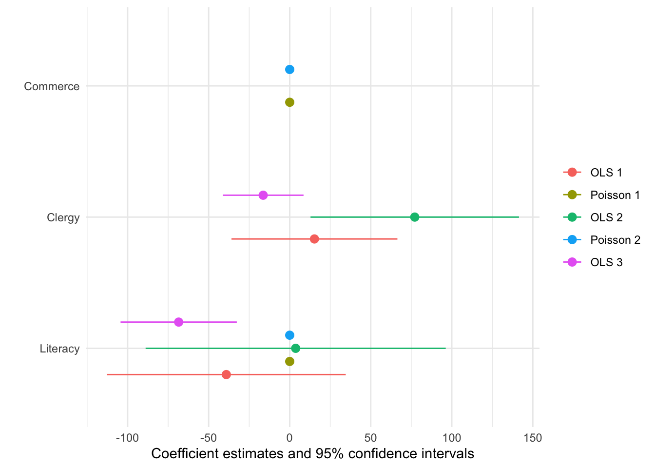

Referecne

• Data and Model Summaries in R
• Model Plots
• citation("modelsummary")