![]()
Regularization Penalized Regression
1 Introduction
1.1 Motivation
The motivation for employing regularization in linear models arises from several contemporary challenges in data analysis:
- High Dimensionality:
- Many modern datasets feature a vast number of variables, sometimes matching or even exceeding the number of observations. This phenomenon is known as high dimensionality. Such datasets are not uncommon in fields like genomics, finance, and image recognition.
- Computational Cost:
- With the increasing scale of data, traditional methods like best subset selection and stepwise feature selection become computationally expensive. For instance, finding an optimal subset in large datasets might require hours of computation, even with high-speed computers.
- Advancements in Techniques:
- Over the past two decades, newer techniques have been developed and refined. These methods surpass the predictive power and interpretability of the linear models discussed in earlier chapters, providing more efficient and scalable solutions.
1.2 Multicollinearity
Data Collection: Sometimes, data are collected from a narrow subspace of the independent variables, creating multicollinearity through the sampling method, which might not exist in the population. Obtaining more data over an expanded range can mitigate this issue.
Overdefined Models: Situations where there are more variables than observations can lead to multicollinearity. This should generally be avoided.
Model Specification: Using powers or interactions of the original variables as new predictors can introduce multicollinearity, especially if the sampling subspace of the independent variables is narrow.
Outliers: Extreme values or outliers in the X-space can induce and mask multicollinearity. This is referred to as multicollinearity caused by outliers and should be corrected by removing outliers before applying techniques like ridge regression.
Regularization serves as a crucial technique in modern statistical modeling, offering a practical approach to handle high-dimensional data and multicollinearity, while enhancing the predictive performance of linear models.
1.3 Regularization Overview
Regularization techniques adjust the coefficients of linear regression models to prevent overfitting, potentially reducing some coefficients to zero. Key regularization methods include:
- Ridge Regression: Adds a penalty equal to the square of the magnitude of coefficients.
- Lasso (Least Absolute Shrinkage and Selection Operator): Penalizes the absolute value of the regression coefficients.
- Elastic Net: Combines penalties of both ridge and lasso regression, allowing for a balance between variable selection and multicollinearity.
The general form of a regularized linear regression model can be expressed as: \[Y ≈ β_0 + β_1X_1 + β_2X_2 + …+ β_pX_p\]
During the fitting process, the objective is to minimize the Residual Sum of Squares (RSS), which measures the difference between observed and predicted values: \[\text{RSS} = \sum _{i=1}^{n}(y_{i}-f(x_{i}))^{2} = \sum _{i=1}^{n}(\varepsilon _{i})^{2}=\sum _{i=1}^{n}(y_{i}-(\alpha +\beta x_{i}))^{2}\]
Regularization introduces a shrinkage penalty to the minimization of RSS. This penalty is controlled by the tuning parameter λ: \[y = β_0 + β_1x_1 + β_2x_2 + … + β_kx_k + λ(\text{slope})²\] When λ = 0, the model reduces to ordinary least squares (OLS) regression, as the regularization term has no effect.
Strengths of Regularization
Computational Efficiency: Regularization is computationally efficient compared to best subset selection, which would require testing \(2^p\) models on a large dataset. Regularization only requires fitting a single model for each value of λ.
Bias-Variance Tradeoff: In linear models, when the relationship between the response and predictor variables is nearly linear, least squares estimates are almost unbiased but can have high variance. This means small changes in the training data can cause large variations in the least squares estimates. Regularization optimally adjusts the bias-variance tradeoff, improving model performance by appropriately selecting λ and the form of regularization.
Multicollinearity: Regularization can address issues of multicollinearity, which arises when predictor variables are highly correlated. This can distort the estimates of the coefficients, making the model sensitive to changes in the model specifications.
2 Model Selection
2.1 Data Preparation
- lcavol: logarithm of tumor volume
- lweight: logarithm of prostate weight
- age: patient age in years
- lbph: logarithm of benign prostatic hyperplasia (BPH), non-cancerous prostatic hyperplasia.
- svi: seminal vesicle invasion, an indicator variable indicating whether cancer cells have penetrated the prostate wall and invaded the seminal vesicle (1=yes, 0=no).
- lcp: logarithm of capsule penetration, indicating the extent to which cancer cells have spread beyond the prostate capsule.
- gleason: the patient’s Gleason score; given by a pathologist after a biopsy (2-10), indicating the degree of mutation of the cancer cells - the higher the score, the more dangerous it is.
- pgg45: the percentage of patients with a Gleason score of 4 or 5 (high-grade cancer).
- lpsa: logarithm of the PSA value, the response variable.
- train: a logical vector (TRUE or FALSE, used to distinguish between training data and test data)
# library(car)      # package to calculate Variance Inflation Factor
# library(corrplot) # correlation plots
# library(leaps)    # best subsets regression
# library(glmnet)   # allows ridge regression, LASSO and elastic net
# library(caret)    # this will help identify the appropriate parameters

prostate <- read.delim("./01_Datasets/prostate.txt", header=T)
# Graphs or tables to understand the data

# As you can see, there is indeed a clear linear relationship between the outcome variable lpsa and the predictor variable lcavol
plot(prostate)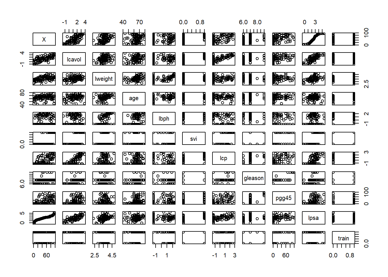
# Create a graph specifically for the feature Gleason
plot(prostate$gleason, ylab = "Gleason Score")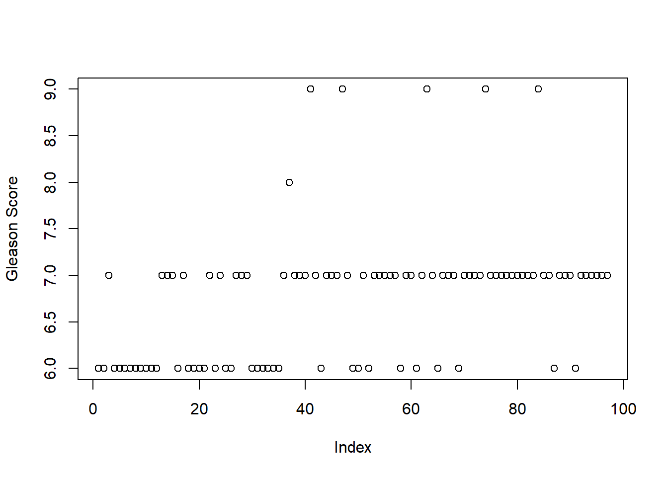
table(prostate$gleason)##
## 6 7 8 9
## 35 56 1 5# Solution
# Delete this feature completely;
# Delete only those scores with values of 8.0 and 9.0;
# Recode the feature to create an indicator variable.
# Creating a box plot with Gleason Score on the horizontal axis and Log of PSA on the vertical axis will help us make our choice
# The best option is to convert this feature into an indicator variable, with 0 representing a score of 6 and 1 representing a score of 7 or higher. Removing the feature may lose the predictive power of the model. Missing values may also cause problems in the glmnet package we will use.
boxplot(prostate$lpsa ~ prostate$gleason, xlab = "Gleason Score",
ylab = "Log of PSA")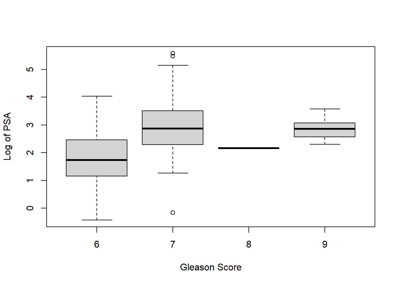
# Use ifelse() command to encode indicator variables
prostate$gleason <- ifelse(prostate$gleason == 6, 0, 1)
table(prostate$gleason)
##
## 0 1
## 35 62# Correlation statistics, indicating whether there is correlation or dependence between features
# Problem found: PSA and logarithm of tumor volume (lcavol) are highly correlated 0.73, multicollinearity: tumor volume is also related to capsule penetration, and capsule penetration is also related to seminal vesicle invasion
p.cor = cor(prostate[,-1])
corrplot.mixed(p.cor)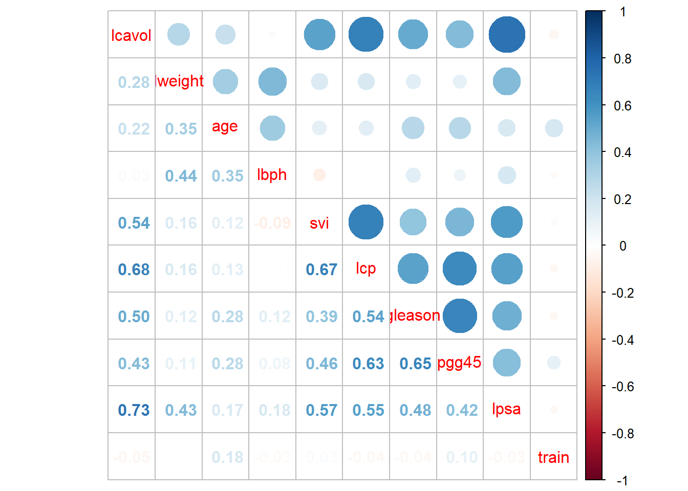
# Before starting machine learning, you must first create a training data set and a test data set
# There is already a feature in the observation that indicates whether the observation belongs to the training set, so we can use the subset() command to divide the observations with a train value of TRUE into In the training set, the observations with train value FALSE are assigned to the test set
train <- subset(prostate, train == TRUE)[, 2:10]
str(train)
## 'data.frame': 67 obs. of 9 variables:
## $ lcavol : num -0.58 -0.994 -0.511 -1.204 0.751 ...
## $ lweight: num 2.77 3.32 2.69 3.28 3.43 ...
## $ age : int 50 58 74 58 62 50 58 65 63 63 ...
## $ lbph : num -1.39 -1.39 -1.39 -1.39 -1.39 ...
## $ svi : int 0 0 0 0 0 0 0 0 0 0 ...
## $ lcp : num -1.39 -1.39 -1.39 -1.39 -1.39 ...
## $ gleason: num 0 0 1 0 0 0 0 0 0 1 ...
## $ pgg45 : int 0 0 20 0 0 0 0 0 0 30 ...
## $ lpsa : num -0.431 -0.163 -0.163 -0.163 0.372 ...test = subset(prostate, train==FALSE)[,2:10]
str(test)## 'data.frame': 30 obs. of 9 variables:
## $ lcavol : num 0.737 -0.777 0.223 1.206 2.059 ...
## $ lweight: num 3.47 3.54 3.24 3.44 3.5 ...
## $ age : int 64 47 63 57 60 69 68 67 65 54 ...
## $ lbph : num 0.615 -1.386 -1.386 -1.386 1.475 ...
## $ svi : int 0 0 0 0 0 0 0 0 0 0 ...
## $ lcp : num -1.386 -1.386 -1.386 -0.431 1.348 ...
## $ gleason: num 0 0 0 1 1 0 0 1 0 0 ...
## $ pgg45 : int 0 0 0 5 20 0 0 20 0 0 ...
## $ lpsa : num 0.765 1.047 1.047 1.399 1.658 ...2.2 Best subset regression
# Create a minimum subset object using the regsubsets() command
subfit <- regsubsets(lpsa ~ ., data = train)
b.sum <- summary(subfit)
# Using the Bayesian Information Criterion, the three-feature model has the smallest BIC value
which.min(b.sum$bic)
## [1] 3# Use a statistical plot to see the relationship between model performance and subset combinations
plot(b.sum$bic, type = "l", xlab = "# of Features", ylab = "BIC",
main = "BIC score by Feature Inclusion")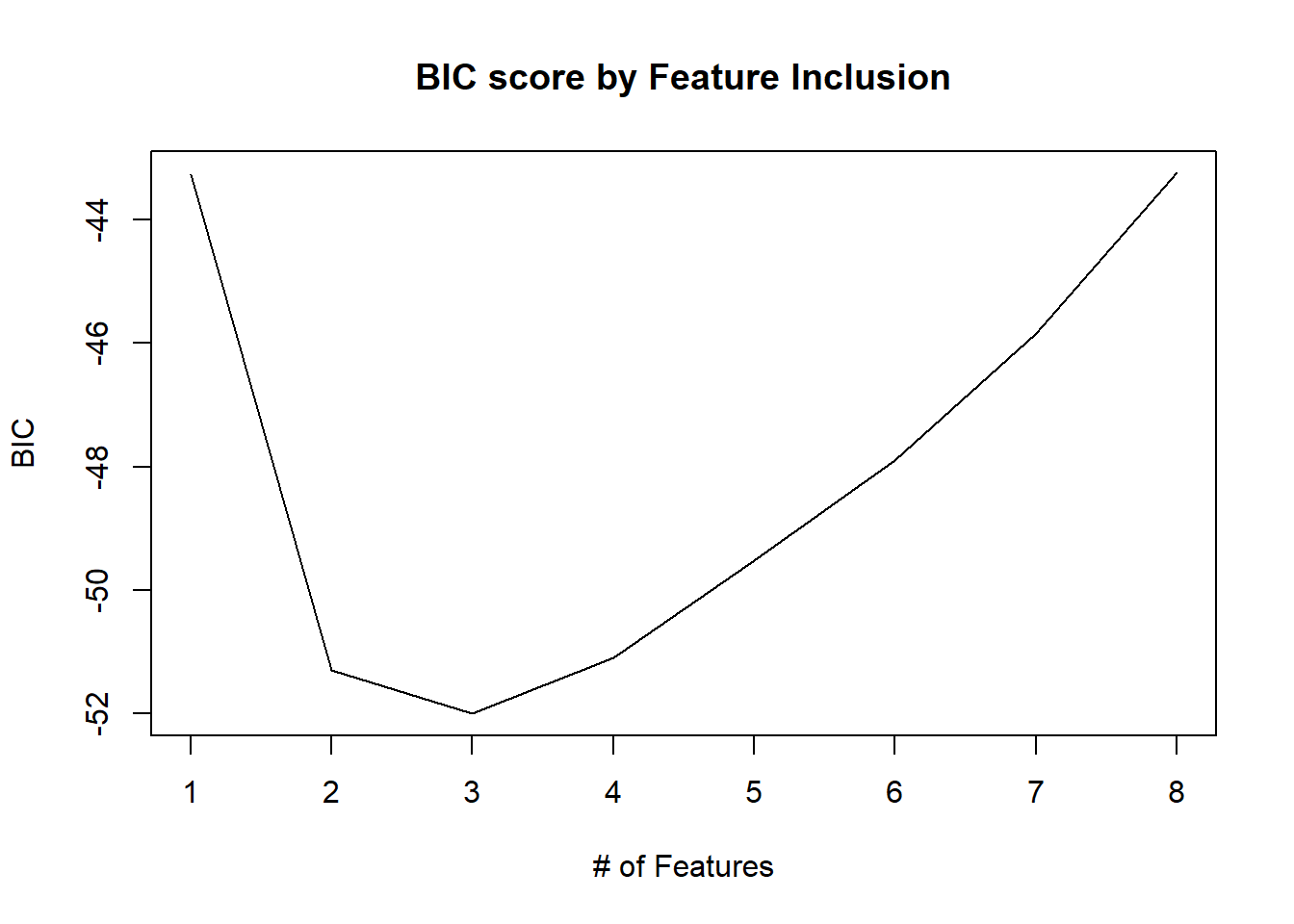
# Make a statistical plot of the actual model for a more detailed inspection. The figure above tells us that the three features in the model with the smallest BIC value are: lcavol, lweight, and gleason
plot(subfit, scale = "bic", main = "Best Subset Features")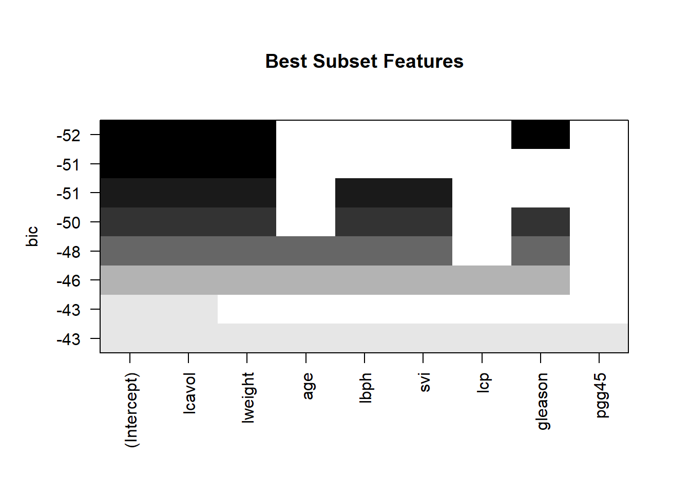
# Use the above three variables to create a linear model
ols <- lm(lpsa ~ lcavol + lweight + gleason, data = train)
# The linear fit is good and there is no heteroskedasticity
plot(ols$fitted.values, train$lpsa, xlab = "Predicted", ylab = "Actual",
main = "Predicted vs Actual")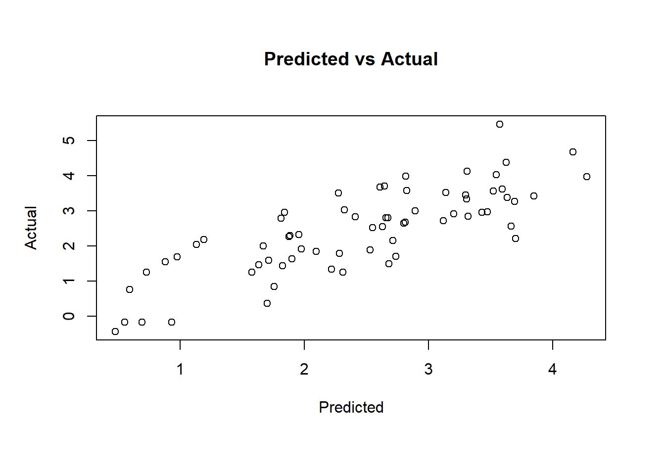
# Model performance on the test set
pred.subfit = predict(ols, newdata=test)
plot(pred.subfit, test$lpsa , xlab = "Predicted",
ylab = "Actual", main = "Predicted vs Actual")
# Calculate the mean squared error MSE to compare between different model building techniques
resid.subfit = test$lpsa - pred.subfit
mean(resid.subfit^2)
## [1] 0.50841263 Ridge Regression
3.1 Introduction
Ridge regression, also referred to as Tikhonov regularization, is designed to handle issues of multicollinearity among predictors in regression models by introducing a bias into the estimates. This method improves upon ordinary least squares (OLS) by incorporating a penalty term to the loss function, typically the L2-norm, which is the sum of the squares of the coefficients.
The primary objective in ridge regression is to minimize the residual sum of squares (RSS) along with an additional penalty term, λ(sumβj²). This term adjusts the coefficients towards zero but not exactly to zero, which helps in reducing the variance of the estimates and prevents overfitting, especially in scenarios where predictor variables are highly correlated. However, because coefficients are shrunk towards zero but never fully eliminated, ridge regression does not inherently perform feature selection, which may impact the interpretability of the model.
The formulation of ridge regression was notably advanced by Hoerl and Kennard in 1970. They proposed a solution to the instability in the OLS estimates that occurs when the matrix \(X'X\) is near-singular (nearly collinear predictors). Their method modifies the ordinary least squares estimator, given by: \[ \hat{\beta}=\left(X^{\prime} X\right)^{-1} X^{\prime} Y, \] by adding a small constant value, λ, to the diagonal entries of \(X'X\) prior to its inversion, thus stabilizing the inversion process. This leads to the ridge estimator: \[ \hat{\beta}_{\text{ridge}} = \left(X^{\prime} X + \lambda I_{p}\right)^{-1} X^{\prime} Y, \] where \(I_p\) is the identity matrix, and λ serves as the regularization parameter. The ridge estimator minimizes: \[ \sum_{i=1}^{n}\left(y_{i}-\sum_{j=1}^{p} x_{i j} \beta_{j}\right)^{2} + \lambda \sum_{j=1}^{p} \beta_{j}^{2}. \] This is equivalent to minimizing the RSS under the constraint that the sum of the squared coefficients remains below a certain threshold. This constraint effectively limits the magnitude of the regression coefficients, promoting smaller and more stable estimates, which can significantly enhance the model’s prediction accuracy and robustness against multicollinearity.
Furthermore, when λ = 0, the ridge estimate reduces to the OLS estimate, illustrating how ridge regression extends OLS by allowing for regularization to manage ill-conditioned data or highly correlated predictors. As λ increases, the bias in the estimates increases, but the variance decreases, providing a trade-off between bias and variance, thus potentially enhancing the model’s predictive performance at the cost of losing some interpretability due to the non-zero shrinkage of all coefficients.
3.2 Property
Based on the information from the image you uploaded, here is a detailed explanation in English of the three properties of ridge regression estimates:
Property 1: Bias of the Ridge Estimator
The ridge estimator \(\hat{\beta}(k)\) introduces a bias to the coefficients compared to the ordinary least squares (OLS) estimator. This bias arises from the penalty term, which shrinks the coefficients towards zero as a function of the regularization parameter \(k\). The expected value of the ridge estimator can be described as: \[ E[\hat{\beta}(k)] = E[(X'X + kI)^{-1}X'Y] = (X'X + kI)^{-1}X'X\beta \] When \(k = 0\), the ridge estimator reduces to the OLS estimator, \(E[\hat{\beta}(0)] = \beta\). However, for \(k > 0\), the estimator exhibits bias, as it pulls the coefficients towards zero. The term \((X'X + kI)^{-1}X'X\) acts to decrease each coefficient’s magnitude, making the ridge estimator biased but potentially more stable in the presence of multicollinearity.
Property 2: Variance of the Ridge Estimator
Ridge regression also affects the variance of the estimator. The variance of the ridge estimator tends to be lower than that of the OLS estimator due to the shrinkage effect. This shrinkage reduces the influence of individual data points and lessens the model’s sensitivity to noise in the data, leading to a lower variance of the estimates: \[ Var[\hat{\beta}(k)] = (X'X + kI)^{-1}X'X(X'X + kI)^{-1} \sigma^2 \] This equation shows that as \(k\) increases, the overall variance of the estimator decreases, trading off some bias for reduced variance.
Property 3: Norm and Mean Squared Error (MSE)
The norm of the ridge estimator \(||\hat{\beta}(k)||\) is always less than or equal to the norm of the OLS estimator \(||\beta||\) as long as \(k > 0\). This property stems from the constraint imposed by the regularization term, which inherently limits the size of the coefficients’ vector, reducing the complexity of the model: \[ ||\hat{\beta}(k)|| \leq ||\beta|| \] Additionally, the MSE of the ridge estimator is generally lower than that of the OLS estimator when \(k > 0\). This reduction in MSE is due to the balance between the increase in bias and the decrease in variance: \[ MSE[\hat{\beta}(k)] < MSE[\hat{\beta}] \] As \(k\) increases from zero, the MSE initially decreases until it reaches a minimum, after which it may start to increase if \(k\) is too large. This behavior highlights the importance of selecting an appropriate value of \(k\) to optimize the trade-off between bias and variance, aiming to achieve the best generalization performance of the ridge regression model.
3.3 Ridge Trace Analysis
Ridge trace analysis is a graphical technique used in ridge regression to select the optimal regularization parameter, typically denoted as \(\lambda\) or \(k\). This method involves plotting how regression coefficients change with different values of the regularization parameter. The purpose of ridge trace analysis is to help analysts find a balance between bias and variance in the model, thus enhancing the model’s prediction accuracy and stability.
Steps and Objectives of Ridge Trace Analysis:
- Choosing a Range of \(\lambda\) Values:
- Ridge trace analysis begins by choosing a range of relatively large \(\lambda\) values and gradually decreasing them. This range should be extensive enough to show how coefficients shrink from their least squares estimates down to near zero.
- Plotting the Coefficients:
- For each value of \(\lambda\), the corresponding set of regression coefficients is calculated. These coefficients are then plotted on a graph, with \(\lambda\) on the x-axis (often on a log scale) and the coefficient values on the y-axis.
- Analyzing the Ridge Trace:
- The resulting plot, known as a “ridge trace”, shows the trajectory of each coefficient as \(\lambda\) increases. Analysts look for a point where the coefficients stabilize before they start to approach zero too closely. This point indicates a good trade-off between reducing the model’s complexity (and hence its variance) and retaining enough flexibility to capture the underlying data patterns without introducing significant bias.
- Selecting the Optimal \(\lambda\):
- The optimal value of \(\lambda\) is typically chosen where the coefficients have stabilized on the ridge trace. This value is critical because it represents where the model is neither too complex (overfitting) nor too simple (underfitting), providing a robust generalization performance.
- Validation:
- To confirm the effectiveness of the chosen \(\lambda\), it is often validated through techniques like cross-validation. This further ensures that the model performs well on unseen data, minimizing the prediction error.
Ridge trace analysis is particularly valuable in scenarios with multicollinearity among predictors or when the number of predictors is high relative to the number of observations. By providing a clear visual of how each \(\lambda\) affects the coefficients, it aids in making informed decisions about the level of regularization that best suits the specific characteristics of the data.
3.4 Selection of Ridge Parameter
Based on the content in the images you provided, there are three key methods outlined for selecting the ridge parameter (\(k\) or \(\lambda\)) in ridge regression. These methods are crucial for optimizing the balance between bias and variance in the model, thereby enhancing model accuracy and stability.
- Choice of \(k\) value range: It is essential to test a wide range of \(k\) values to ensure that the entire spectrum of model behaviors is considered. Often, a logarithmic scale is used for \(k\) to explore both very small and larger values comprehensively.
- Stability of \(k\): In all methods, it is crucial to look for stability in the choice of \(k\). A small change in \(k\) should not lead to a large change in the coefficients or the MSE, suggesting that the chosen \(k\) is robust.
1. Ridge Trace Analysis
Ridge trace analysis involves plotting the coefficients of the regression variables against different values of the regularization parameter \(k\). By visually inspecting these plots, one can determine the best value of \(k\) by identifying the point where the coefficients stabilize before becoming too small or converging towards zero. This method is especially useful for seeing how each predictor is affected by changes in \(k\) and choosing a \(k\) that keeps all important variables in a stable range without over-shrinking them.
2. Generalized Cross-Validation (GCV)
Generalized Cross-Validation (GCV) is a more systematic approach that involves evaluating the model’s predictive performance for different values of \(k\). The objective is to select a \(k\) that minimizes the GCV score, which is an estimate of the model’s prediction error. This method automatically accounts for the trade-off between fit and complexity (model variance and bias), making it highly effective for datasets where direct validation through splitting may be impractical due to size constraints.
3. Minimization of Mean Squared Error (MSE)
This method focuses on the mean squared error associated with different \(k\) values. By calculating or estimating the MSE for a range of \(k\) values and selecting the \(k\) that minimizes this MSE, one can theoretically find the optimal balance between bias (due to underfitting) and variance (due to overfitting). The MSE can be calculated directly from the training data, or more robustly, it can be estimated via cross-validation to ensure the chosen \(k\) generalizes well to new data.
3.5 Modeling using
glmnet
The glmnet package in R is a powerful and efficient tool
for fitting generalized linear models (GLMs) with regularization,
specifically ridge regression and LASSO (Least Absolute Shrinkage and
Selection Operator). It is widely used for handling high-dimensional
data, where the number of predictors is large, and multicollinearity or
sparsity is present. Regularization techniques like ridge and LASSO help
improve model accuracy and stability by adding penalty terms to the loss
function.
Flexibility with Regularization:
- Ridge regression (\(\alpha = 0\)): Shrinks the coefficients towards zero without eliminating any predictors.
- LASSO (\(\alpha = 1\)): Performs variable selection by shrinking some coefficients to exactly zero.
- Elastic Net (\(0 < \alpha < 1\)): Combines the benefits of ridge and LASSO by applying both L2 and L1 penalties.
Automatic Standardization:
- By default,
glmnetstandardizes the input variables (mean 0, variance 1) before fitting the model to ensure that the penalty is applied uniformly across all predictors. After fitting, the coefficients are returned in their original, unstandardized scale.
- By default,
Efficient Computation:
- The package implements efficient algorithms for calculating solutions across a range of penalty values (\(\lambda\)) in a single function call, making it computationally efficient.
x <- as.matrix(train[, 1:8])
y <- train[, 9]
ridge <- glmnet(x, y, family = "gaussian", alpha = 0)
print(ridge)
##
## Call: glmnet(x = x, y = y, family = "gaussian", alpha = 0)
##
## Df %Dev Lambda
## 1 8 0.00 878.90
## 2 8 0.56 800.80
## 3 8 0.61 729.70
## 4 8 0.67 664.80
## 5 8 0.74 605.80
## 6 8 0.81 552.00
## 7 8 0.89 502.90
## 8 8 0.97 458.20
## 9 8 1.07 417.50
## 10 8 1.17 380.40
## 11 8 1.28 346.60
## 12 8 1.40 315.90
## 13 8 1.54 287.80
## 14 8 1.68 262.20
## 15 8 1.84 238.90
## 16 8 2.02 217.70
## 17 8 2.21 198.40
## 18 8 2.42 180.70
## 19 8 2.64 164.70
## 20 8 2.89 150.10
## 21 8 3.16 136.70
## 22 8 3.46 124.60
## 23 8 3.78 113.50
## 24 8 4.13 103.40
## 25 8 4.50 94.24
## 26 8 4.91 85.87
## 27 8 5.36 78.24
## 28 8 5.84 71.29
## 29 8 6.36 64.96
## 30 8 6.93 59.19
## 31 8 7.54 53.93
## 32 8 8.19 49.14
## 33 8 8.90 44.77
## 34 8 9.65 40.79
## 35 8 10.46 37.17
## 36 8 11.33 33.87
## 37 8 12.25 30.86
## 38 8 13.24 28.12
## 39 8 14.28 25.62
## 40 8 15.39 23.34
## 41 8 16.55 21.27
## 42 8 17.78 19.38
## 43 8 19.07 17.66
## 44 8 20.41 16.09
## 45 8 21.81 14.66
## 46 8 23.27 13.36
## 47 8 24.77 12.17
## 48 8 26.31 11.09
## 49 8 27.90 10.10
## 50 8 29.51 9.21
## 51 8 31.15 8.39
## 52 8 32.81 7.64
## 53 8 34.47 6.96
## 54 8 36.14 6.35
## 55 8 37.80 5.78
## 56 8 39.45 5.27
## 57 8 41.08 4.80
## 58 8 42.68 4.37
## 59 8 44.24 3.99
## 60 8 45.76 3.63
## 61 8 47.24 3.31
## 62 8 48.66 3.02
## 63 8 50.03 2.75
## 64 8 51.34 2.50
## 65 8 52.60 2.28
## 66 8 53.80 2.08
## 67 8 54.93 1.89
## 68 8 56.01 1.73
## 69 8 57.03 1.57
## 70 8 58.00 1.43
## 71 8 58.91 1.30
## 72 8 59.76 1.19
## 73 8 60.57 1.08
## 74 8 61.33 0.99
## 75 8 62.04 0.90
## 76 8 62.70 0.82
## 77 8 63.33 0.75
## 78 8 63.91 0.68
## 79 8 64.45 0.62
## 80 8 64.96 0.56
## 81 8 65.43 0.51
## 82 8 65.87 0.47
## 83 8 66.28 0.43
## 84 8 66.66 0.39
## 85 8 67.01 0.35
## 86 8 67.33 0.32
## 87 8 67.63 0.29
## 88 8 67.90 0.27
## 89 8 68.15 0.24
## 90 8 68.38 0.22
## 91 8 68.59 0.20
## 92 8 68.77 0.18
## 93 8 68.94 0.17
## 94 8 69.09 0.15
## 95 8 69.23 0.14
## 96 8 69.35 0.13
## 97 8 69.46 0.12
## 98 8 69.55 0.11
## 99 8 69.64 0.10
## 100 8 69.71 0.09# The Y axis is the coefficient value, the X axis is the L1 norm, and the figure shows the relationship between the coefficient value and the L1 norm
plot(ridge, label = TRUE)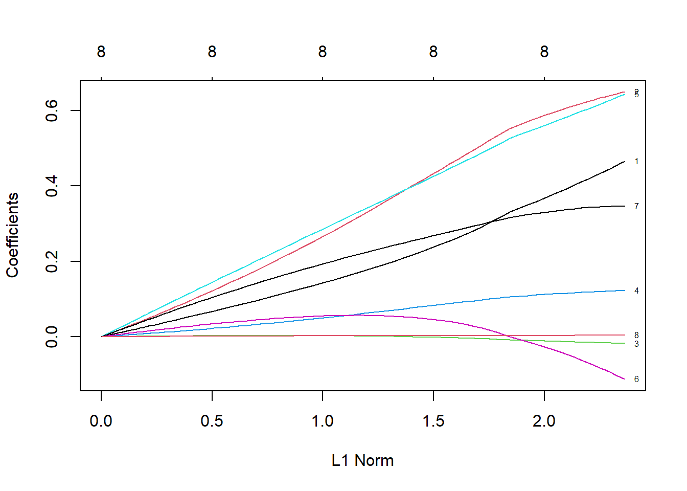
# See how the coefficient value changes with the change of λ
plot(ridge, xvar = "lambda", label = TRUE)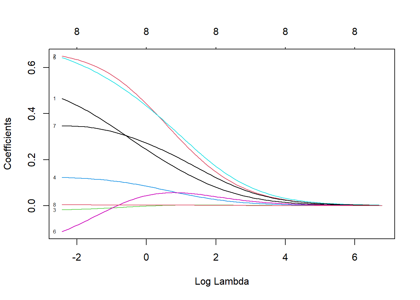
# See how the coefficient value changes with the percentage of explained deviation, replace lamda with dev
# When λ decreases, the coefficient will increase, and the percentage of explained deviation will also increase. If the lambda value is set to 0, the shrinkage penalty will be ignored and the model will be equivalent to OLS
plot(ridge, xvar = "dev", label = TRUE)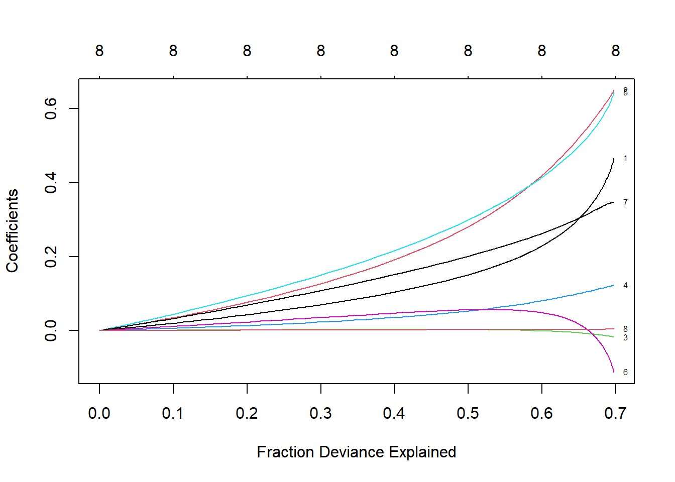
# Prove it on the test set
newx <- as.matrix(test[, 1:8])
ridge.y = predict(ridge, newx = newx, type = "response", s=0.1)
# Draw a statistical graph showing the relationship between predicted values and actual values
plot(ridge.y, test$lpsa, xlab = "Predicted",
ylab = "Actual", main = "Ridge Regression")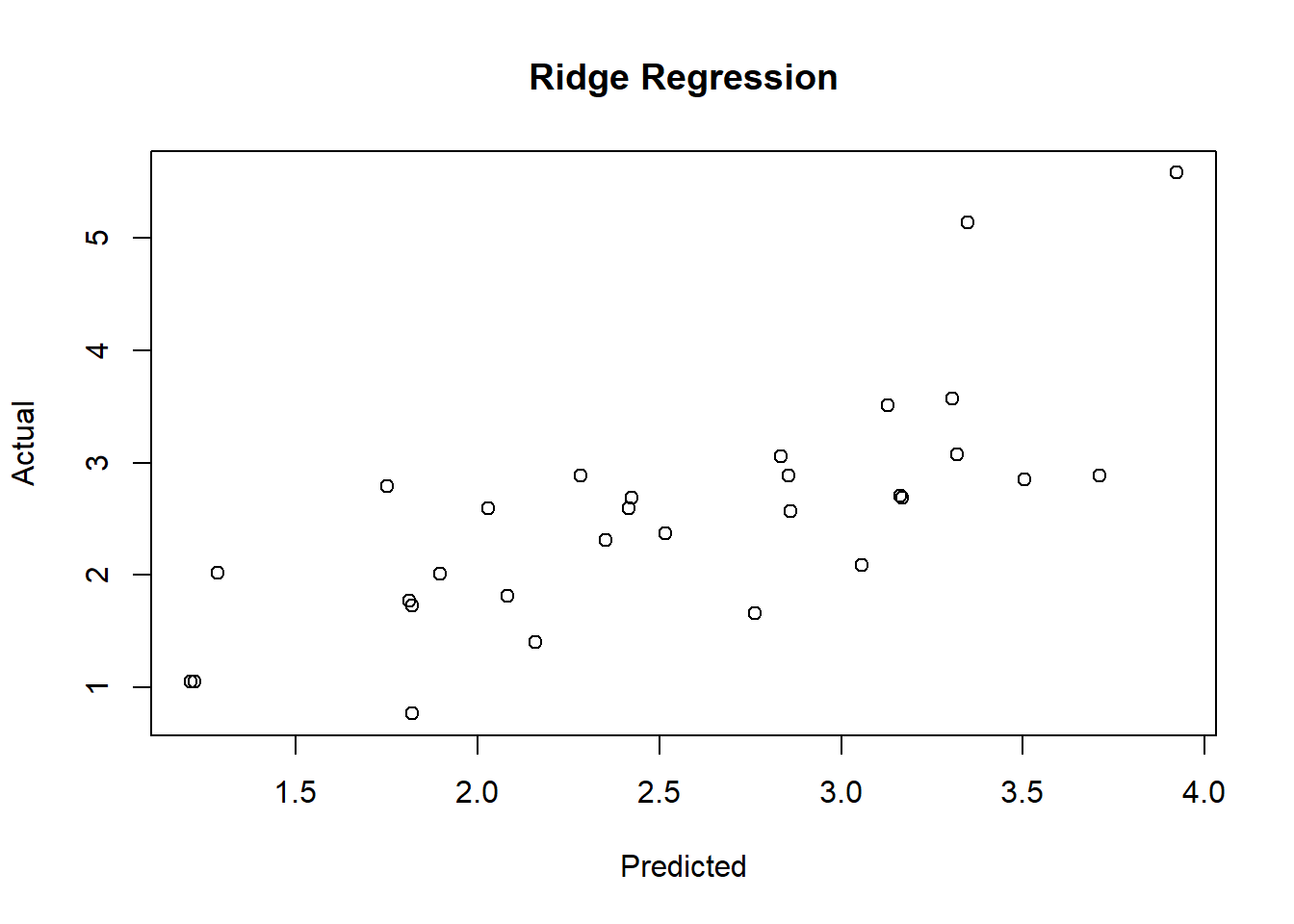
# Calculate MSE
ridge.resid <- ridge.y - test$lpsa
mean(ridge.resid^2)
## [1] 0.47835594 Lasso Regression
4.1 Introduction
区别于岭回归中的L2-norm,LASSO使用L1-norm,即所有特征权重的绝对值之和, 也就是要最小化RSS + λ(sum|βj|)。这个收缩惩罚项确实可以使特征权重收缩到0. 相对于岭回归,这是 L2-norm 一个明显的优势,因为可以极大地提高模型的解释性。 但是,存在高共线性或高度两两相关 的情况下,LASSO可能会将某个预测特征强制删除,这会损失模型的预测能力. 如果 特征A和B都应该存在于模型之中,那么LASSO可能会将其中一个的系数缩减到0。
如果较少数目的预测变量有实际系数,其余预测变量的系数要么非常小,要么为0, 那么在这样的情况下,LASSO性能更好。 当响应变量是很多预测变量的函数,而且预测变量的系数大小都差不多时,岭回归表现得更好 两全其美的机会: 弹性网络既能做到岭回归不能做的特征提取,也能实现LASSO不能做的 特征分组。
A ridge solution can be hard to interpret because it is not sparse (no \(\beta\) ’s are set exactly to 0 ).
- Ridge subject to: \(\sum_{j=1}^{p}\left(\beta_{j}\right)^{2}<c\).
- Lasso subject to: \(\sum_{j=1}^{p}\left|\beta_{j}\right|<c\).
This is a subtle, but important change. Some of the coefficients may be shrunk exactly to zero. The least absolute shrinkage and selection operator, or lasso, as described in Tibshirani (1996) is a technique that has received a great deal of interest. As with ridge regression we assume the covariates are standardized. Lasso estimates of the coefficients (Tibshirani, 1996) achieve min \((Y-X \beta)^{\prime}(Y-X \beta)+\lambda \sum_{j=1}^{p}\left|\beta_{j}\right|\), so that the L2 penalty of ridge regression \(\sum_{j=1}^{p} \beta_{j}^{2}\) is replaced by an L1 penalty, \(\sum_{j=1}^{p}\left|\beta_{j}\right|\).
4.2 Modeling using
glmnet
lasso <- glmnet(x, y, family = "gaussian", alpha = 1)
print(lasso)
##
## Call: glmnet(x = x, y = y, family = "gaussian", alpha = 1)
##
## Df %Dev Lambda
## 1 0 0.00 0.87890
## 2 1 9.13 0.80080
## 3 1 16.70 0.72970
## 4 1 22.99 0.66480
## 5 1 28.22 0.60580
## 6 1 32.55 0.55200
## 7 1 36.15 0.50290
## 8 1 39.14 0.45820
## 9 2 42.81 0.41750
## 10 2 45.98 0.38040
## 11 3 48.77 0.34660
## 12 3 51.31 0.31590
## 13 4 53.49 0.28780
## 14 4 55.57 0.26220
## 15 4 57.30 0.23890
## 16 4 58.74 0.21770
## 17 4 59.93 0.19840
## 18 5 61.17 0.18070
## 19 5 62.20 0.16470
## 20 5 63.05 0.15010
## 21 5 63.76 0.13670
## 22 5 64.35 0.12460
## 23 5 64.84 0.11350
## 24 5 65.24 0.10340
## 25 6 65.58 0.09424
## 26 6 65.87 0.08587
## 27 6 66.11 0.07824
## 28 6 66.31 0.07129
## 29 7 66.63 0.06496
## 30 7 66.96 0.05919
## 31 7 67.24 0.05393
## 32 7 67.46 0.04914
## 33 7 67.65 0.04477
## 34 8 67.97 0.04079
## 35 8 68.34 0.03717
## 36 8 68.66 0.03387
## 37 8 68.92 0.03086
## 38 8 69.13 0.02812
## 39 8 69.31 0.02562
## 40 8 69.46 0.02334
## 41 8 69.58 0.02127
## 42 8 69.68 0.01938
## 43 8 69.77 0.01766
## 44 8 69.84 0.01609
## 45 8 69.90 0.01466
## 46 8 69.95 0.01336
## 47 8 69.99 0.01217
## 48 8 70.02 0.01109
## 49 8 70.05 0.01010
## 50 8 70.07 0.00921
## 51 8 70.09 0.00839
## 52 8 70.11 0.00764
## 53 8 70.12 0.00696
## 54 8 70.13 0.00635
## 55 8 70.14 0.00578
## 56 8 70.15 0.00527
## 57 8 70.15 0.00480
## 58 8 70.16 0.00437
## 59 8 70.16 0.00399
## 60 8 70.17 0.00363
## 61 8 70.17 0.00331
## 62 8 70.17 0.00301
## 63 8 70.17 0.00275
## 64 8 70.18 0.00250
## 65 8 70.18 0.00228
## 66 8 70.18 0.00208
## 67 8 70.18 0.00189
## 68 8 70.18 0.00172
## 69 8 70.18 0.00157# 模型构建过程在69步之后停止了,因为解释偏差不再随着λ值的增加而减小。还要 注意,Df列现在也随着λ变化。初看上去,当λ值为0.001572时,所有8个特征都应该包括在模型 中。然而,出于测试的目的,我们先用更少特征的模型进行测试,比如7特征模型。从下面的结 果行中可以看到,λ值大约为0.045时,模型从7个特征变为8个特征。因此,使用测试集评价模型 时要使用这个λ值
plot(lasso, xvar = "lambda", label = TRUE)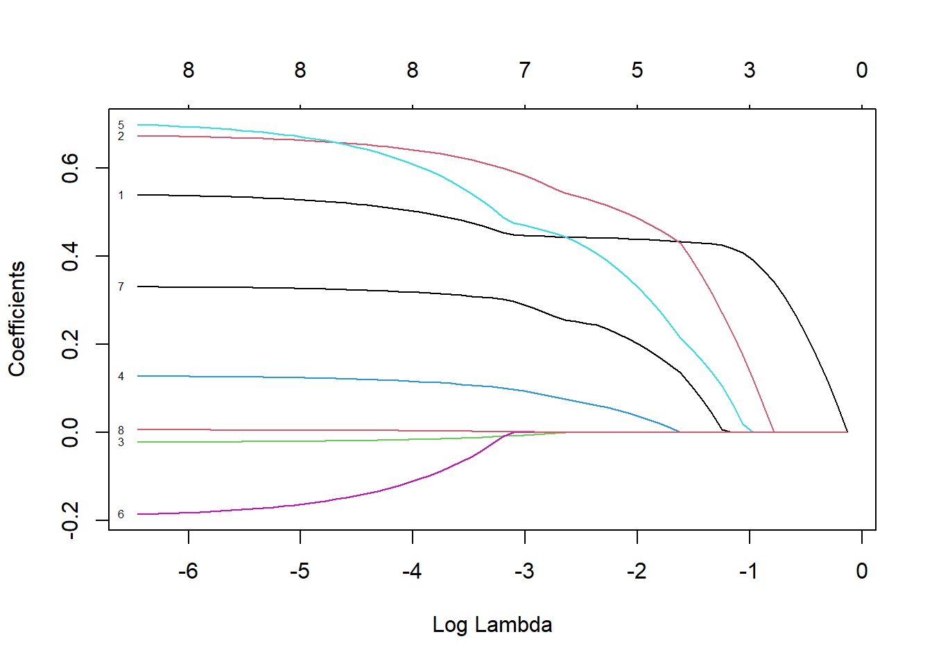
lasso.coef <- coef(lasso, s = 0.045)
lasso.coef
## 9 x 1 sparse Matrix of class "dgCMatrix"
## s1
## (Intercept) -0.1305900670
## lcavol 0.4479592050
## lweight 0.5910476764
## age -0.0073162861
## lbph 0.0974103575
## svi 0.4746790830
## lcp .
## gleason 0.2968768129
## pgg45 0.0009788059# LASSO算法在λ值为0.045时,将lcp的系数归零
# LASSO模型在测试集上的表现
lasso.y <- predict(lasso, newx = newx,
type = "response", s = 0.045)
plot(lasso.y, test$lpsa, xlab = "Predicted", ylab = "Actual",
main = "LASSO")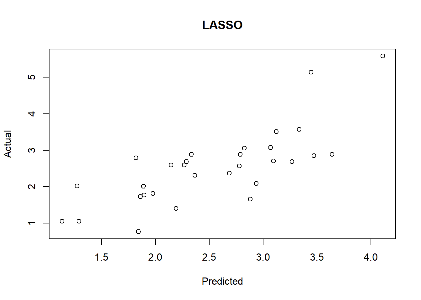
lasso.resid <- lasso.y - test$lpsa
mean(lasso.resid^2)
## [1] 0.44372094.3 glmnet cross validation
glmnet包在使用cv.glmnet()估计 λ值时,默认使用10折交叉验证。 在K折交叉验证中,数据被划分成k个相同的子集(折),每次使 用k 1个子集拟合模型,然后使用剩下的那个子集做测试集,最后将k次拟合的结果综合起来(一 般取平均数),确定最后的参数。
# 3折交叉验证
set.seed(317)
lasso.cv = cv.glmnet(x, y, nfolds = 3)
plot(lasso.cv)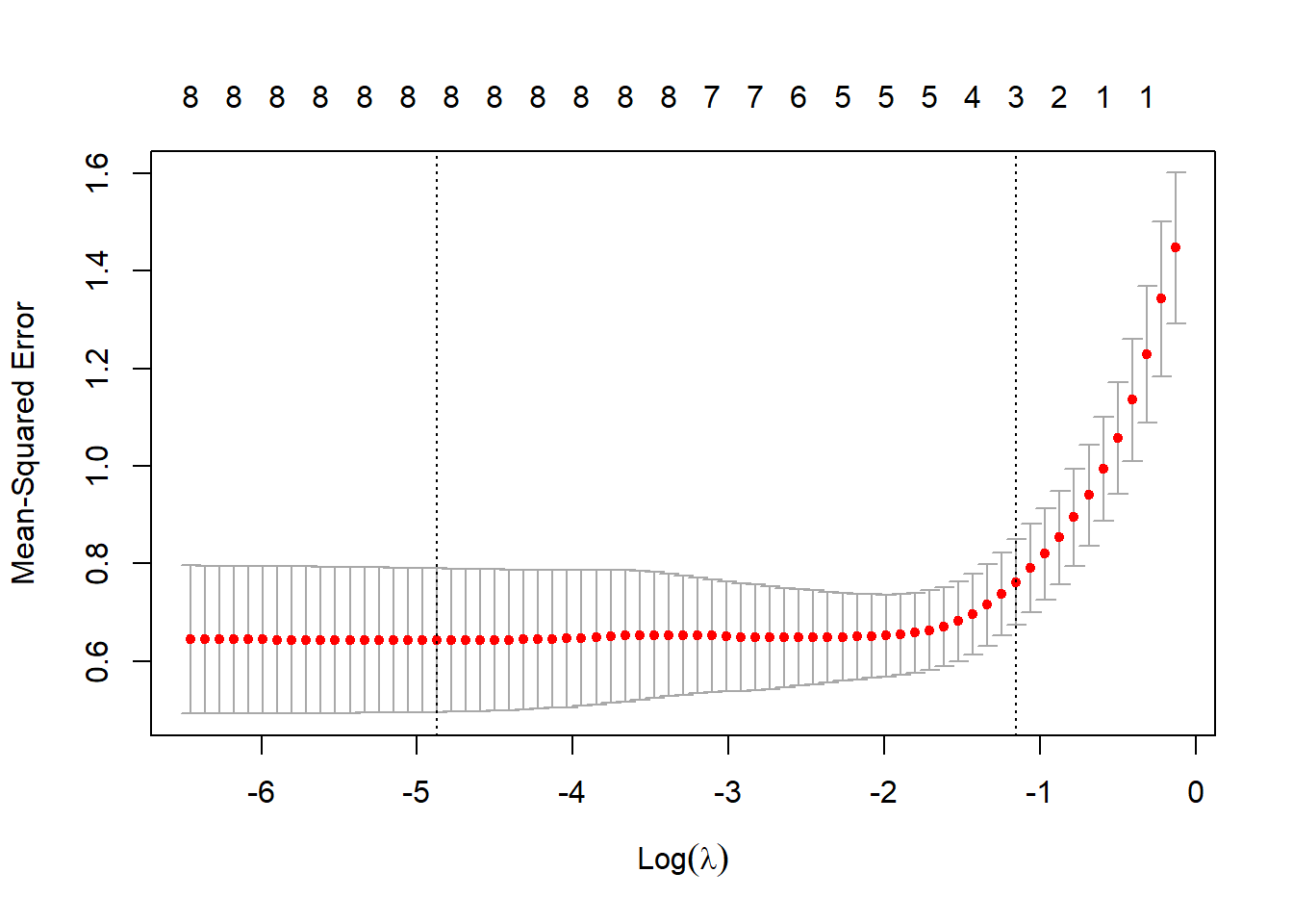
# Interpretation
# CV统计图和glmnet中其他统计图有很大区别,它表示λ的对数值和均方误差之间的关系,还 带有模型中特征的数量。图中两条垂直的虚线表示取得MSE最小值的logλ(左侧虚线)和距离最 小值一个标准误差的logλ。如果有过拟合问题,那么距离最小值一个标准误的位置是非常好的解决问题的起点。

# 得到这两个λ的具体值
lasso.cv$lambda.min # minimum
## [1] 0.007644054lasso.cv$lambda.1se # one standard error away## [1] 0.3158532# 查看系数并在测试集上进行模型验证
# 模型的误差为0.45,只有5个特征,排除了age、lcp和pgg45
coef(lasso.cv, s = "lambda.1se")## 9 x 1 sparse Matrix of class "dgCMatrix"
## s1
## (Intercept) 1.07462462
## lcavol 0.41767273
## lweight 0.22464383
## age .
## lbph .
## svi 0.06489231
## lcp .
## gleason .
## pgg45 .lasso.y.cv = predict(lasso.cv, newx=newx, type = "response",
s = "lambda.1se")
lasso.cv.resid = lasso.y.cv - test$lpsa
mean(lasso.cv.resid^2)## [1] 0.55082645 ElasticNet
弹性网络(ElasticNet)
- 既能做到岭回归不能做的特征提取,也能实现LASSO不能做的 特征分组。
- LASSO倾向于在一组相关的特征中选择一个,忽略其他。弹性网络包含了 一个混合参数α,它和λ同时起作用。 α是一个0和1之间的数,λ和前面一样,用来调节惩罚项的大小。 当α等于0时,弹性网络等价于岭回归;当α等于1时,弹性网络等价于LASSO。
- 实质上,通过对β系数的二次项引入一个第二调优参数,将L1惩罚项和L2惩罚项混合在一起。 通过最小化(RSS + λ[(1-α)(sum|βj|2)/2 + α(sum|βj|)]/N)完成目标。
5.1 Modeling using
glmnet
弹性网络参数α。回忆一下,α = 0表示岭回归惩罚,α = 1表示LASSO惩罚, 弹性网络参数为0≤α≤1。同时解出两个不同的参数会非常麻烦,求助于R中的老朋友——caret包。
caret包旨在解决分类问题和训练回归模型,它配有一个很棒的网站,帮助人们掌握其所有功能:http://topepo.github.io/caret/index.html
- 使用R基础包中的expand.grid()函数,建立一个向量存储我们要研究的α和λ的所有 组合。
- 使用caret包中的trainControl()函数确定重取样方法,像第2章一样,使用LOOCV。
- P在caret包的train()函数中使用glmnet()训练模型来选择α和λ。
规则试验: * α从0到1,每次增加0.2;请记住,α被绑定在0和1之间。 * λ从0到0.20,每次增加0.02;0.2的λ值是岭回归λ值(λ = 0.1)和LASSOλ值(λ = 0.045)之间的一个中间值。 * expand.grid()函数建立这个向量并生成一系列数值,caret包会自动使用这些数值
grid <- expand.grid(.alpha = seq(0,1, by=.2),
                    .lambda = seq(0.00, 0.2, by = 0.02))
table(grid)
## .lambda
## .alpha 0 0.02 0.04 0.06 0.08 0.1 0.12 0.14 0.16 0.18 0.2
## 0 1 1 1 1 1 1 1 1 1 1 1
## 0.2 1 1 1 1 1 1 1 1 1 1 1
## 0.4 1 1 1 1 1 1 1 1 1 1 1
## 0.6 1 1 1 1 1 1 1 1 1 1 1
## 0.8 1 1 1 1 1 1 1 1 1 1 1
## 1 1 1 1 1 1 1 1 1 1 1 1head(grid)# 对于定量型响应变量,使用算法的默认选择均方根误差即可完美实现
control <- trainControl(method = "LOOCV") # selectionFunction="best"
set.seed(701) # our random seed
enet.train = train(lpsa ~ ., data = train,
method = "glmnet",
trControl = control,
tuneGrid = grid)
enet.train## glmnet
##
## 67 samples
## 8 predictor
##
## No pre-processing
## Resampling: Leave-One-Out Cross-Validation
## Summary of sample sizes: 66, 66, 66, 66, 66, 66, ...
## Resampling results across tuning parameters:
##
## alpha lambda RMSE Rsquared MAE
## 0.0 0.00 0.7498311 0.6091434 0.5684548
## 0.0 0.02 0.7498311 0.6091434 0.5684548
## 0.0 0.04 0.7498311 0.6091434 0.5684548
## 0.0 0.06 0.7498311 0.6091434 0.5684548
## 0.0 0.08 0.7498311 0.6091434 0.5684548
## 0.0 0.10 0.7508038 0.6079576 0.5691343
## 0.0 0.12 0.7512303 0.6073484 0.5692774
## 0.0 0.14 0.7518536 0.6066518 0.5694451
## 0.0 0.16 0.7526409 0.6058786 0.5696155
## 0.0 0.18 0.7535502 0.6050559 0.5699154
## 0.0 0.20 0.7545583 0.6041945 0.5709377
## 0.2 0.00 0.7550170 0.6073913 0.5746434
## 0.2 0.02 0.7542648 0.6065770 0.5713633
## 0.2 0.04 0.7550427 0.6045111 0.5738111
## 0.2 0.06 0.7571893 0.6015388 0.5764117
## 0.2 0.08 0.7603394 0.5978544 0.5793641
## 0.2 0.10 0.7642219 0.5936131 0.5846567
## 0.2 0.12 0.7684937 0.5890900 0.5898445
## 0.2 0.14 0.7713716 0.5861699 0.5939008
## 0.2 0.16 0.7714681 0.5864527 0.5939535
## 0.2 0.18 0.7726979 0.5856865 0.5948039
## 0.2 0.20 0.7744041 0.5845281 0.5959671
## 0.4 0.00 0.7551309 0.6072931 0.5746628
## 0.4 0.02 0.7559055 0.6044693 0.5737468
## 0.4 0.04 0.7599608 0.5989266 0.5794120
## 0.4 0.06 0.7667450 0.5911506 0.5875213
## 0.4 0.08 0.7746900 0.5824231 0.5979116
## 0.4 0.10 0.7760605 0.5809784 0.6001763
## 0.4 0.12 0.7784160 0.5788024 0.6024102
## 0.4 0.14 0.7792216 0.5786250 0.6035698
## 0.4 0.16 0.7784433 0.5806388 0.6024696
## 0.4 0.18 0.7779134 0.5828322 0.6014095
## 0.4 0.20 0.7797721 0.5826306 0.6020934
## 0.6 0.00 0.7553016 0.6071317 0.5748038
## 0.6 0.02 0.7579330 0.6020021 0.5766881
## 0.6 0.04 0.7665234 0.5917067 0.5863966
## 0.6 0.06 0.7778600 0.5790948 0.6021629
## 0.6 0.08 0.7801170 0.5765439 0.6049216
## 0.6 0.10 0.7819242 0.5750003 0.6073379
## 0.6 0.12 0.7800315 0.5782365 0.6053700
## 0.6 0.14 0.7813077 0.5785548 0.6059119
## 0.6 0.16 0.7846753 0.5770307 0.6075899
## 0.6 0.18 0.7886388 0.5753101 0.6104210
## 0.6 0.20 0.7931549 0.5734018 0.6140249
## 0.8 0.00 0.7553734 0.6070686 0.5748255
## 0.8 0.02 0.7603679 0.5991567 0.5797001
## 0.8 0.04 0.7747753 0.5827275 0.5975303
## 0.8 0.06 0.7812784 0.5752601 0.6065340
## 0.8 0.08 0.7832103 0.5734172 0.6092662
## 0.8 0.10 0.7811248 0.5769787 0.6071341
## 0.8 0.12 0.7847355 0.5750115 0.6093756
## 0.8 0.14 0.7894184 0.5725728 0.6122536
## 0.8 0.16 0.7951091 0.5696205 0.6158407
## 0.8 0.18 0.8018475 0.5659672 0.6205741
## 0.8 0.20 0.8090352 0.5622252 0.6256726
## 1.0 0.00 0.7554439 0.6070354 0.5749409
## 1.0 0.02 0.7632577 0.5958706 0.5827830
## 1.0 0.04 0.7813519 0.5754986 0.6065914
## 1.0 0.06 0.7843882 0.5718847 0.6103528
## 1.0 0.08 0.7819175 0.5755415 0.6082954
## 1.0 0.10 0.7860004 0.5731009 0.6107923
## 1.0 0.12 0.7921572 0.5692525 0.6146159
## 1.0 0.14 0.7999326 0.5642789 0.6198758
## 1.0 0.16 0.8089248 0.5583637 0.6265797
## 1.0 0.18 0.8185327 0.5521348 0.6343174
## 1.0 0.20 0.8259445 0.5494268 0.6411104
##
## RMSE was used to select the optimal model using the smallest value.
## The final values used for the model were alpha = 0 and lambda = 0.08.# 选择最优模型的原则是RMSE值最小,模型最后选定的最优参数组合是α = 0,λ = 0.08。
# 实验设计得到的最优调优参数是α = 0和λ = 0.08,相当于glmnet中s = 0.08的岭回归
# 在测试集上验证模型
# enet <- glmnet(x, y,family = "gaussian",
# alpha = 0,
# lambda = .08)
# enet.coef <- coef(enet, s = .08, exact = TRUE)
# enet.coef
# enet.y <- predict(enet, newx = newx, type = "response", s= .08)
# plot(enet.y, test$lpsa, xlab = "Predicted",
# ylab = "Actual", main = "Elastic Net")
# enet.resid <- enet.y - test$lpsa
# mean(enet.resid^2)5.2 Classification
# 用于逻辑斯蒂回归
# 加载准备乳腺癌数据
# library(MASS)
biopsy$ID = NULL
names(biopsy) = c("thick", "u.size", "u.shape", "adhsn",
"s.size", "nucl", "chrom", "n.nuc", "mit", "class")
biopsy.v2 <- na.omit(biopsy)
set.seed(123) #random number generator
ind <- sample(2, nrow(biopsy.v2), replace = TRUE, prob = c(0.7, 0.3))
train <- biopsy.v2[ind==1, ] #the training data set
test <- biopsy.v2[ind==2, ] #the test data set
x <- as.matrix(train[, 1:9])
y <- train[, 10]
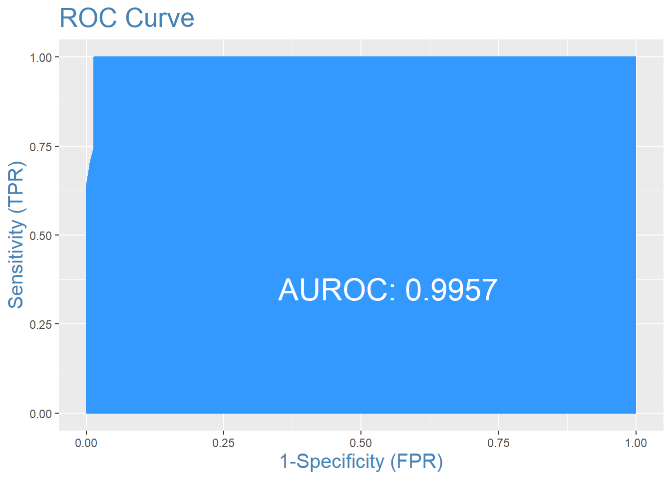
# 函数cv.glmnet中,将family的值设定为binomial,将measure的值设定为曲线下面积 (auc),并使用5折交叉验证
set.seed(3)
fitCV <- cv.glmnet(x, y, family = "binomial",
type.measure = "auc",
nfolds = 5)
# 绘制fitCV,可以看出AUC和λ的关系
plot(fitCV)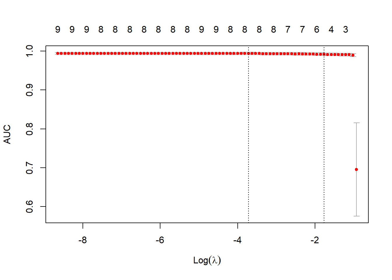
# 模型系数,选择出的5个特征是thickness、u.size、u.shape, nucl, n.nuc
fitCV$lambda.1se
## [1] 0.1710154coef(fitCV, s = "lambda.1se")## 10 x 1 sparse Matrix of class "dgCMatrix"
## s1
## (Intercept) -2.01180454
## thick 0.03320390
## u.size 0.10789382
## u.shape 0.08617195
## adhsn .
## s.size .
## nucl 0.15038212
## chrom .
## n.nuc 0.00483271
## mit .# 通过误差和auc,查看这个模型在测试集上的表现
# library(InformationValue)
predCV <- predict(fitCV, newx = as.matrix(test[, 1:9]),
s = "lambda.1se",
type = "response")
actuals <- ifelse(test$class == "malignant", 1, 0)
misClassError(actuals, predCV)## [1] 0.0574plotROC(actuals, predCV)